9 Correlation
Video introduction to correlation (Italian)
- direct (e.g. Air temperature, daily mean values at two contiguous stations are correlated)
- indirect (heart issues ~ cholesterol)
- …
9.1 Install Packages
install.packages("readxl")  # import excel files
install.packages("ggplot2") # advanced plots
install.packages("GGally") # plot correlation9.4 What is correlation
Correlation is a statistical measure that suggests the level of linear dependence between two variables, that occur in pair – just like what we have here in MODENAURB and SAGATABOAGRO.
Correlation can take values between -1 to +1. If we observe for every instance where MODENAURB increases, the SAGATABOAGRO also increases along with it, then there is a high positive correlation between them and therefore the correlation between them will be closer to 1.
The opposite is true for an inverse relationship, in which case, the correlation between the variables will be close to -1.
A value closer to 0 suggests a weak relationship between the variables.
A low correlation (-0.2 < x < 0.2) probably suggests that much of variation of the response variable (Y) is unexplained by the predictor (X), in which case, we should probably look for better explanatory variables.
Correlation coefficient between two random variables \(X\) and \(Y\) is defined as \[\rho(X,Y) = \frac{{\bf Cov}(X,Y)}{\sqrt{{\bf Var}(X){\bf Var}(Y)}} = \frac{{\bf E}[(X-\mu_x)(Y-\mu_y)]}{{\bf \sigma}(X){\bf \sigma}(Y)}\]
where- Cov is the covariance
- Var is the variance
- \(\mu_x\) is the mean of X
- \(\mu_y\) is the mean of Y
- \({\bf \sigma}(X)\) is the standard deviation of X
- \({\bf \sigma}(Y)\) is the standard deviation of Y
\[{\bf \sigma}(X) = \sqrt{ \frac{\sum_{i=1}^n (y_i - \bar{y})^2}{N} }\]
9.5 An example of application to heigth vs foot size
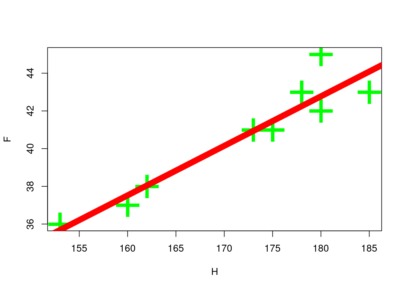
Create an example using the height (H) and foot size (F) of students:
H    <- c(178,180,175,162,153,160,185,173,180,175)
F    <- c(43,45,41,38,36,37,43,41,42,41)
NAME <- c('Giulians','Albert','Stephans','Lucy','Fed','Mary','Federico','Anto','Antonio','Nadir')
9.5.1 Compute Pearson correlation
Calculate sample size(n), mean height (mu_H) and mean foot size (mu_F)
Print the values:
n
#> [1] 10
mu_H
#> [1] 172.1
mu_F
#> [1] 40.7
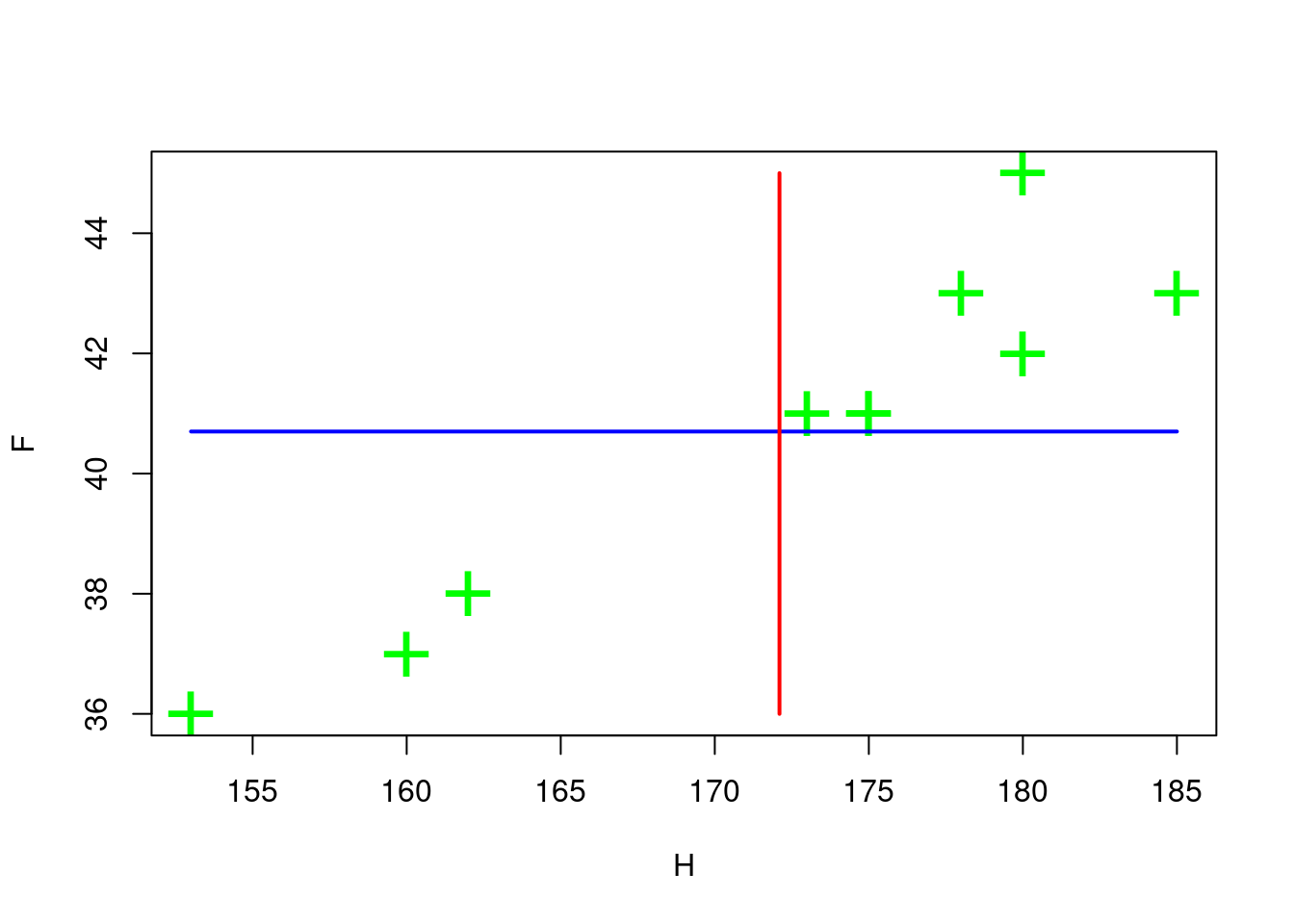
Plot the scatter of points and the average value for each variable
# scatter
plot( H,F,pch='+',col='green', cex=3 )
# plot the line of the mean value of P
lines( H,                  replicate(n,mu_F), col='blue', lwd=2 )
# plot the line of the mean value of H
lines( replicate(n,mu_H) , F,                 col='red' , lwd=2 )
Deviation of heigth:
\(H - \mu_H\)
H - mean(H)
#>  [1]   5.9   7.9   2.9 -10.1 -19.1 -12.1  12.9   0.9   7.9
#> [10]   2.9
NAME
#>  [1] "Giulians" "Albert"   "Stephans" "Lucy"     "Fed"
#>  [6] "Mary"     "Federico" "Anto"     "Antonio"  "Nadir"
Squared Deviation of heigth:
\((H - \mu_H)^2 = (H - \mu_H) \times (H - \mu_H)\)
(H - mean(H))^2
#>  [1]  34.81  62.41   8.41 102.01 364.81 146.41 166.41   0.81
#>  [9]  62.41   8.41
Mean Squared Deviation of heigth:
\(\frac{\sum\limits_{i \in n} (H_i - \mu_H)^2}{n}\)
Mean Squared Deviation of foot size:
The Variance of H is equal to the Mean Squared Deviation of H:
\(Var(H) = \frac{\sum\limits_{i \in n} (H_i - \mu_H)^2}{n} = \frac{\sum\limits_{i \in n} (H_i - \mu_H) \times (H_i - \mu_H) }{n}\)
VAR_H  = sum( (H - mu_H)^2 ) / n
VAR_H
#> [1] 95.69
The Variance of P:
VAR_F  = sum( (F - mu_F)^2 ) / n
VAR_F
#> [1] 7.41
The Covariance of H is equal to the Mean Production of Deviations of H and F:
\(COV(H,F) = \frac{\sum\limits_{i \in n} (H_i - \mu_H)\times (F_i - \mu_F)}{n}\)
COV_HF = sum( (H - mu_H)*(F - mu_F) ) / n
COV_HF
#> [1] 25.13
9.5.2 Create Pearson correlation function
myCorr = function(X,Y){
    nx = length(X)
    ny = length(Y)
    if (nx!=ny){
        stop('The length of inputs is different!')
    }else{
        n = nx
    }
    mu_x   = mean(X)
    mu_y   = mean(Y)
    COV_XY = sum( (X-mu_x)*(Y-mu_y) ) / n
    VAR_X  = sum( (X-mu_x)^2 ) / n
    VAR_Y  = sum( (Y-mu_y)^2 ) / n
    COV_XY / sqrt(VAR_X*VAR_Y) # --> RETURN CORRELATION
}
# it returns an error:
myCorr( H[1:5], F )
#> Error in myCorr(H[1:5], F): The length of inputs is different!
# it returns an error:
cor(H[1:5], F)
#> Error in cor(H[1:5], F): incompatible dimensions
myCorr(H, F)
#> [1] 0.9437351
cor(H, F)
#> [1] 0.9437351
9.6 More examples of application to climatic Data
9.6.1 Import Climatic Data [ \(T_{max}\), Rain ]
Tmax <- read_excel("../datasets/interchange/Tmax.xlsx", sheet = "measurements", na = "NA")
Rain <- read_excel("../datasets/interchange/Rainfall.xlsx", sheet = "measurements", na = "NA")9.6.3 Correlation Matrix
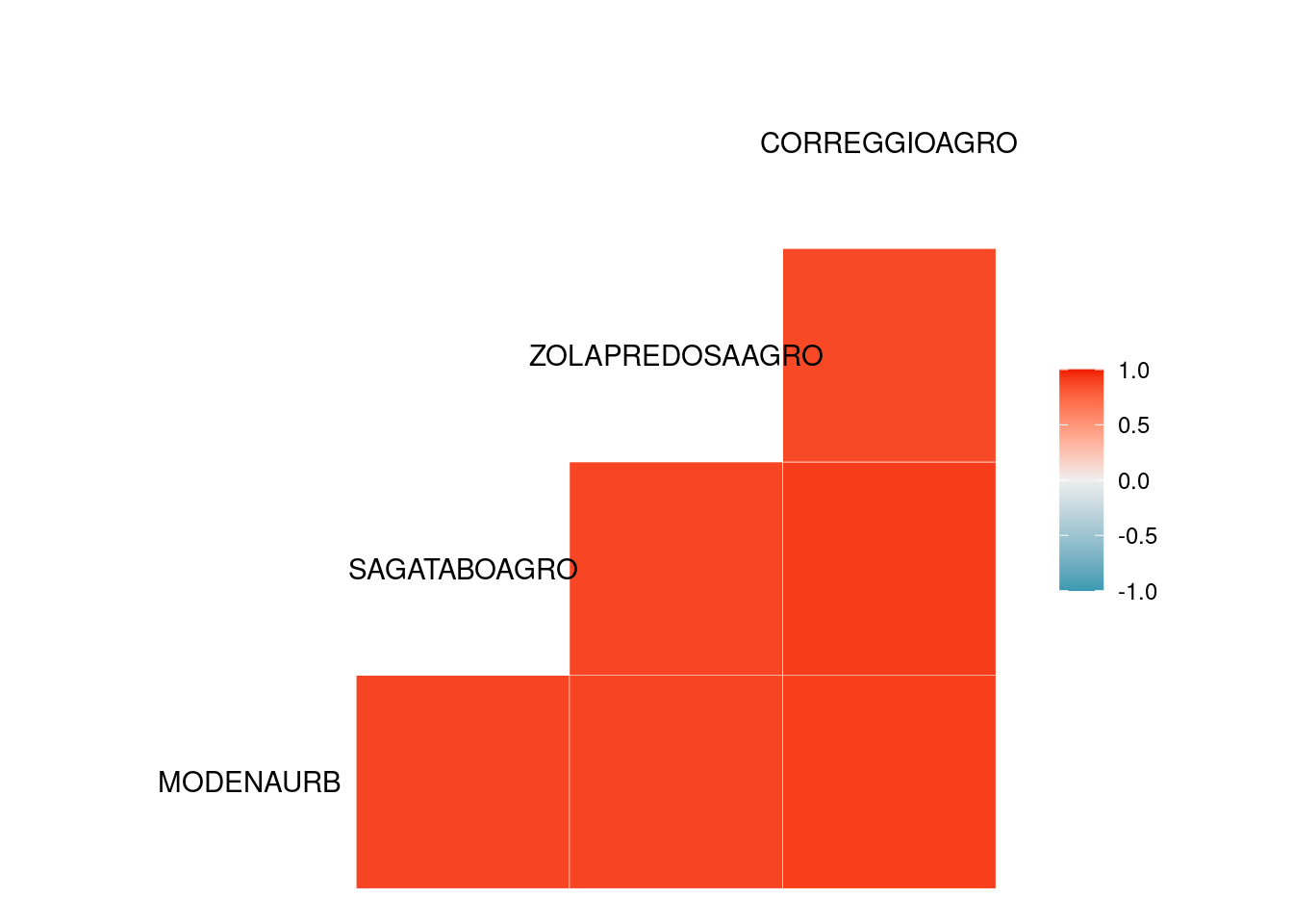
cor(Tmax_jan[,2:6])
#>                 MODENAURB SAGATABOAGRO ZOLAPREDOSAAGRO
#> MODENAURB       1.0000000    0.7604654       0.7621995
#> SAGATABOAGRO    0.7604654    1.0000000       0.8826693
#> ZOLAPREDOSAAGRO 0.7621995    0.8826693       1.0000000
#> RAVARINO               NA           NA              NA
#> CORREGGIOAGRO   0.7136222    0.9164861       0.8699178
#>                 RAVARINO CORREGGIOAGRO
#> MODENAURB             NA     0.7136222
#> SAGATABOAGRO          NA     0.9164861
#> ZOLAPREDOSAAGRO       NA     0.8699178
#> RAVARINO               1            NA
#> CORREGGIOAGRO         NA     1.0000000
cor(Tmax_jan[,2:ncol(Tmax)])
#>                 MODENAURB SAGATABOAGRO ZOLAPREDOSAAGRO
#> MODENAURB       1.0000000    0.7604654       0.7621995
#> SAGATABOAGRO    0.7604654    1.0000000       0.8826693
#> ZOLAPREDOSAAGRO 0.7621995    0.8826693       1.0000000
#> RAVARINO               NA           NA              NA
#> CORREGGIOAGRO   0.7136222    0.9164861       0.8699178
#>                 RAVARINO CORREGGIOAGRO
#> MODENAURB             NA     0.7136222
#> SAGATABOAGRO          NA     0.9164861
#> ZOLAPREDOSAAGRO       NA     0.8699178
#> RAVARINO               1            NA
#> CORREGGIOAGRO         NA     1.0000000
9.6.4 Correlation after removal of measurements
N = 10 # missing values
rows_NA = sample( x=1:31 , size=N , replace=FALSE )
rows_NA
#>  [1] 31 26 29 20  4 22 16 19 17 13
Tmax_jan[rows_NA,2] = NA
Tmax_jan
#> # A tibble: 31 × 6
#>    DATE                MODENAURB SAGATABOAGRO
#>    <dttm>                  <dbl>        <dbl>
#>  1 2007-01-01 00:00:00       6.5          7
#>  2 2007-01-02 00:00:00      10.9         10
#>  3 2007-01-03 00:00:00      13.3         12.9
#>  4 2007-01-04 00:00:00      NA            7
#>  5 2007-01-05 00:00:00      10.5         11.9
#>  6 2007-01-06 00:00:00      10.5         10.7
#>  7 2007-01-07 00:00:00      10.1          9.9
#>  8 2007-01-08 00:00:00       8.2          8.2
#>  9 2007-01-09 00:00:00      10.7         10.7
#> 10 2007-01-10 00:00:00       7.5          6.8
#> # ℹ 21 more rows
#> # ℹ 3 more variables: ZOLAPREDOSAAGRO <dbl>,
#> #   RAVARINO <lgl>, CORREGGIOAGRO <dbl>
cor( Tmax_jan[,2:ncol(Tmax_jan)] , use='pairwise.complete.obs' )
#>                 MODENAURB SAGATABOAGRO ZOLAPREDOSAAGRO
#> MODENAURB       1.0000000    0.8806996       0.8520667
#> SAGATABOAGRO    0.8806996    1.0000000       0.8826693
#> ZOLAPREDOSAAGRO 0.8520667    0.8826693       1.0000000
#> RAVARINO               NA           NA              NA
#> CORREGGIOAGRO   0.9189546    0.9164861       0.8699178
#>                 RAVARINO CORREGGIOAGRO
#> MODENAURB             NA     0.9189546
#> SAGATABOAGRO          NA     0.9164861
#> ZOLAPREDOSAAGRO       NA     0.8699178
#> RAVARINO              NA            NA
#> CORREGGIOAGRO         NA     1.0000000
cor.test(Tmax_jan$MODENAURB,Tmax_jan$SAGATABOAGRO)
#>
#>  Pearson's product-moment correlation
#>
#> data:  Tmax_jan$MODENAURB and Tmax_jan$SAGATABOAGRO
#> t = 8.1045, df = 19, p-value = 1.381e-07
#> alternative hypothesis: true correlation is not equal to 0
#> 95 percent confidence interval:
#>  0.7244320 0.9508762
#> sample estimates:
#>       cor
#> 0.8806996
