5 Raster Data Model
5.2 Load libraries
library(sf)       # vector spatial data classes and functions
library(terra)    # raster spatial data classes and functions
library(tmap)     # noninteractive and interactive maps
library(stars)    # spatiotemporal arrays classes and functions
library(ggplot2)  # non-spatial and spatial plotting
library(units)    # units conversions
5.3 Schematic representation of a raster
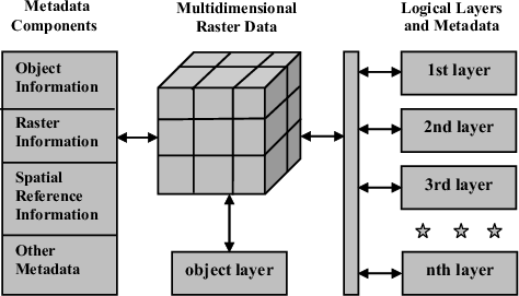
5.3.3 Raster data & metadata
We can distinguish two blocks in a raster (also called grid):
-
metadata, such as
- class, e.g. SpatRaster, (OLD: RasterLayer)
- size, e.g. 3264 x 4800 pixels (nrows x ncols)
- resolution, e.g. 5 meters (synonims are CELLSIZE, PIXELSIZE)
- extent / bounding box (xmin, xmax, ymin, ymax)
- crs (a geographic or projected coordinate system, generally in the proj4 format or EPSG code)
- no data value, e.g. -9999 (synonims are NODATAVALUE, NODATA)
- source (location of file on hard disk, such as ../docente_Langella/Raster-Data/dem5m_vt.tif)
-
data, that is a matrix (=grid) of cells (=pixels)
- the grid of cells has size nrows x ncols
- each cell in a grid store one numeric value (e.g. integer or double number)
- (we can have multiple layers as depicted in the multidimensional raster data representaion)
5.4 Import raster | example: D.E.M.
The command ?rast search for raster string in the documentation.
If the terra package is not loaded in R, the command below gives a warning that nothing was found.
?rastLoad the terra package in R
The command below open the documentation of the rast() function of the terra package in the help:
?rast
getwd()
#> [1] "/home/giuliano/lectures"
5.4.1 Import (i.e. read) a raster
One of the most common rasters used worldwide is the one storing the elevation of each point of land surface.
This kind of raster is called D.E.M., that is Digital Elevation Model.
The raster has the data matrix in which each pixel stores the value of elevation of that surface on Earth.
Any time we are interested in reading a geodata (raster or vector) we need three diferent information:
- path to the file (e.g.
../datasets/raster/), - file name (
dem5m_vt), - file extension (
tif), use a point to separate the filename and the extension.
dem <- rast("../datasets/raster/dem5m_vt.tif")
class(dem)
#> [1] "SpatRaster"
#> attr(,"package")
#> [1] "terra"
hasValues(dem)
#> [1] TRUE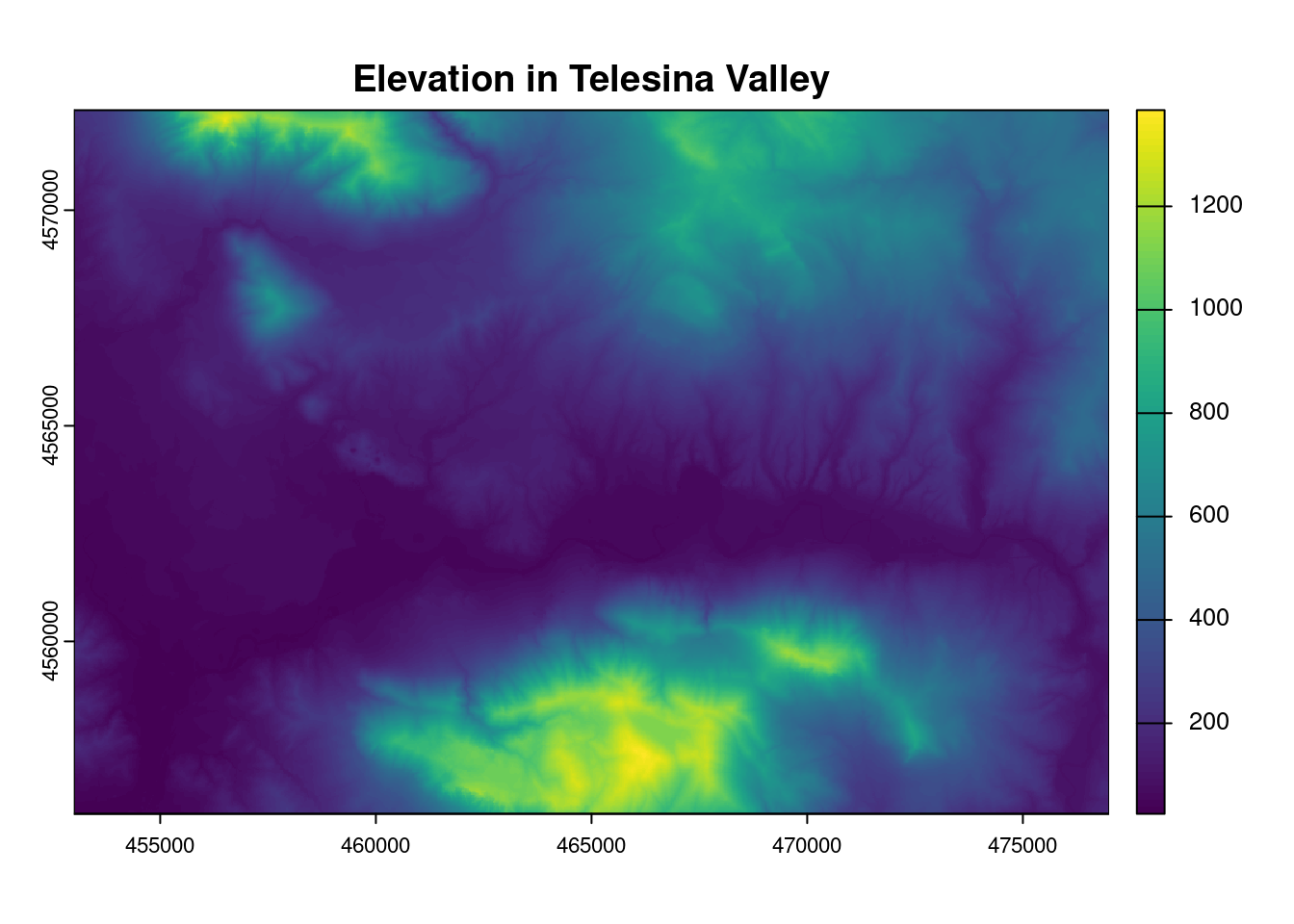
5.4.2 Metadata
5.4.2.1 Print the dem metadata
dem
#> class       : SpatRaster
#> dimensions  : 3264, 4800, 1  (nrow, ncol, nlyr)
#> resolution  : 5, 5  (x, y)
#> extent      : 453000, 477000, 4556000, 4572320  (xmin, xmax, ymin, ymax)
#> coord. ref. : WGS 84 / UTM zone 33N (EPSG:32633)
#> source      : dem5m_vt.tif
#> name        : dem5m_vt
5.4.2.2 Extent
ext(dem)
#> SpatExtent : 453000, 477000, 4556000, 4572320 (xmin, xmax, ymin, ymax)
5.4.2.3 Bounding Box
st_bbox(dem)
#>    xmin    ymin    xmax    ymax
#>  453000 4556000  477000 4572320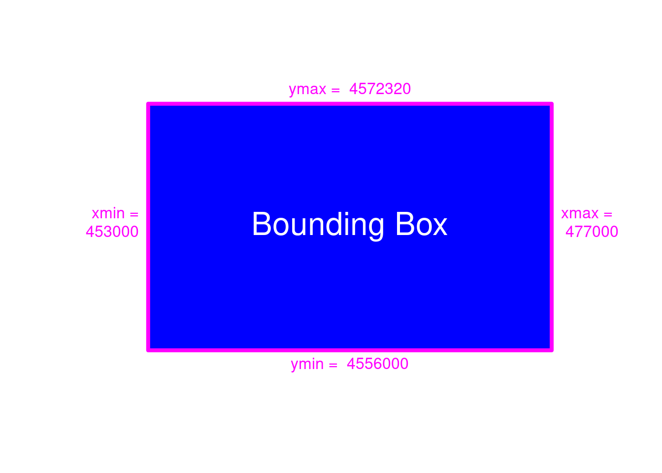
Figure 5.3: Bounding Box Visualization
ymax(dem)
#> [1] 4572320
5.4.2.4 Pixelsize or (spatial) resolution
res(dem)
#> [1] 5 5
5.4.2.5 How many rows are in the height of the bounding box?
Written using the metadata from the print of dem above:
(4572320 - 4556000)/5
#> [1] 3264
Written using the R object dem called by dedicated functions > ymax() , ymin() , res()
5.4.2.6 About the Coordinate Reference System\(\ldots\)
Using terra::crs:
terra::crs(dem)  # {terra}
#> [1] "PROJCRS[\"WGS 84 / UTM zone 33N\",\n    BASEGEOGCRS[\"WGS 84\",\n        ENSEMBLE[\"World Geodetic System 1984 ensemble\",\n            MEMBER[\"World Geodetic System 1984 (Transit)\"],\n            MEMBER[\"World Geodetic System 1984 (G730)\"],\n            MEMBER[\"World Geodetic System 1984 (G873)\"],\n            MEMBER[\"World Geodetic System 1984 (G1150)\"],\n            MEMBER[\"World Geodetic System 1984 (G1674)\"],\n            MEMBER[\"World Geodetic System 1984 (G1762)\"],\n            MEMBER[\"World Geodetic System 1984 (G2139)\"],\n            ELLIPSOID[\"WGS 84\",6378137,298.257223563,\n                LENGTHUNIT[\"metre\",1]],\n            ENSEMBLEACCURACY[2.0]],\n        PRIMEM[\"Greenwich\",0,\n            ANGLEUNIT[\"degree\",0.0174532925199433]],\n        ID[\"EPSG\",4326]],\n    CONVERSION[\"UTM zone 33N\",\n        METHOD[\"Transverse Mercator\",\n            ID[\"EPSG\",9807]],\n        PARAMETER[\"Latitude of natural origin\",0,\n            ANGLEUNIT[\"degree\",0.0174532925199433],\n            ID[\"EPSG\",8801]],\n        PARAMETER[\"Longitude of natural origin\",15,\n            ANGLEUNIT[\"degree\",0.0174532925199433],\n            ID[\"EPSG\",8802]],\n        PARAMETER[\"Scale factor at natural origin\",0.9996,\n            SCALEUNIT[\"unity\",1],\n            ID[\"EPSG\",8805]],\n        PARAMETER[\"False easting\",500000,\n            LENGTHUNIT[\"metre\",1],\n            ID[\"EPSG\",8806]],\n        PARAMETER[\"False northing\",0,\n            LENGTHUNIT[\"metre\",1],\n            ID[\"EPSG\",8807]]],\n    CS[Cartesian,2],\n        AXIS[\"(E)\",east,\n            ORDER[1],\n            LENGTHUNIT[\"metre\",1]],\n        AXIS[\"(N)\",north,\n            ORDER[2],\n            LENGTHUNIT[\"metre\",1]],\n    USAGE[\n        SCOPE[\"Navigation and medium accuracy spatial referencing.\"],\n        AREA[\"Between 12°E and 18°E, northern hemisphere between equator and 84°N, onshore and offshore. Austria. Bosnia and Herzegovina. Cameroon. Central African Republic. Chad. Congo. Croatia. Czechia. Democratic Republic of the Congo (Zaire). Gabon. Germany. Hungary. Italy. Libya. Malta. Niger. Nigeria. Norway. Poland. San Marino. Slovakia. Slovenia. Svalbard. Sweden. Vatican City State.\"],\n        BBOX[0,12,84,18]],\n    ID[\"EPSG\",32633]]"
Note: if you use the cat() function to print the previous command, you’ll get the same result as given below. Please, try it!
Using sf::st_crs:
sf::st_crs(dem)  # {sf}
#> Coordinate Reference System:
#>   User input: WGS 84 / UTM zone 33N
#>   wkt:
#> PROJCRS["WGS 84 / UTM zone 33N",
#>     BASEGEOGCRS["WGS 84",
#>         ENSEMBLE["World Geodetic System 1984 ensemble",
#>             MEMBER["World Geodetic System 1984 (Transit)"],
#>             MEMBER["World Geodetic System 1984 (G730)"],
#>             MEMBER["World Geodetic System 1984 (G873)"],
#>             MEMBER["World Geodetic System 1984 (G1150)"],
#>             MEMBER["World Geodetic System 1984 (G1674)"],
#>             MEMBER["World Geodetic System 1984 (G1762)"],
#>             MEMBER["World Geodetic System 1984 (G2139)"],
#>             ELLIPSOID["WGS 84",6378137,298.257223563,
#>                 LENGTHUNIT["metre",1]],
#>             ENSEMBLEACCURACY[2.0]],
#>         PRIMEM["Greenwich",0,
#>             ANGLEUNIT["degree",0.0174532925199433]],
#>         ID["EPSG",4326]],
#>     CONVERSION["UTM zone 33N",
#>         METHOD["Transverse Mercator",
#>             ID["EPSG",9807]],
#>         PARAMETER["Latitude of natural origin",0,
#>             ANGLEUNIT["degree",0.0174532925199433],
#>             ID["EPSG",8801]],
#>         PARAMETER["Longitude of natural origin",15,
#>             ANGLEUNIT["degree",0.0174532925199433],
#>             ID["EPSG",8802]],
#>         PARAMETER["Scale factor at natural origin",0.9996,
#>             SCALEUNIT["unity",1],
#>             ID["EPSG",8805]],
#>         PARAMETER["False easting",500000,
#>             LENGTHUNIT["metre",1],
#>             ID["EPSG",8806]],
#>         PARAMETER["False northing",0,
#>             LENGTHUNIT["metre",1],
#>             ID["EPSG",8807]]],
#>     CS[Cartesian,2],
#>         AXIS["(E)",east,
#>             ORDER[1],
#>             LENGTHUNIT["metre",1]],
#>         AXIS["(N)",north,
#>             ORDER[2],
#>             LENGTHUNIT["metre",1]],
#>     USAGE[
#>         SCOPE["Navigation and medium accuracy spatial referencing."],
#>         AREA["Between 12°E and 18°E, northern hemisphere between equator and 84°N, onshore and offshore. Austria. Bosnia and Herzegovina. Cameroon. Central African Republic. Chad. Congo. Croatia. Czechia. Democratic Republic of the Congo (Zaire). Gabon. Germany. Hungary. Italy. Libya. Malta. Niger. Nigeria. Norway. Poland. San Marino. Slovakia. Slovenia. Svalbard. Sweden. Vatican City State."],
#>         BBOX[0,12,84,18]],
#>     ID["EPSG",32633]]
5.4.3 Data
5.4.4 Extract
Calculate the mean X and Y of the bounding box of the DEM above, which can be also considered as the center of gravity of the DEM.
Average coordinates:
Xmean
#> [1] 465000
Ymean
#> [1] 4564160
Extract the elevation value for the DEM center of gravity:
Now analyse the situation from the point of view of the row-column dem subsetting.
This instruction selects the upper-left pixel of the 2x2 pixel box centered on the center of gravity:
Indeed, the same value provided by the extract function is returned selecting the lower-right pixel of the 2x2 pixel box centered on the center of gravity (see +1):
5.4.4.0.1 Exercise
Fulfil the assignment given at Raster geodata > Extract
5.5 Create new raster from scratch
5.5.1 We must provide Bounding Box, resolution and CRS
GRID <- rast( xmin = 453000,
              xmax = 477000,
              ymin = 4556000,
              ymax = 4572320,
              resolution = 25,
              crs = "epsg:32633")
Print the metadata of the raster created above:
GRID
#> class       : SpatRaster
#> dimensions  : 653, 960, 1  (nrow, ncol, nlyr)
#> resolution  : 25, 25  (x, y)
#> extent      : 453000, 477000, 4556000, 4572325  (xmin, xmax, ymin, ymax)
#> coord. ref. : WGS 84 / UTM zone 33N (EPSG:32633)
Remove the CRS:
crs(GRID) <- NULLCheck the CRS:
GRID
#> class       : SpatRaster
#> dimensions  : 653, 960, 1  (nrow, ncol, nlyr)
#> resolution  : 25, 25  (x, y)
#> extent      : 453000, 477000, 4556000, 4572325  (xmin, xmax, ymin, ymax)
#> coord. ref. :
Define a CRS:
crs(GRID) <- "epsg:32633"Check the CRS again:
GRID
#> class       : SpatRaster
#> dimensions  : 653, 960, 1  (nrow, ncol, nlyr)
#> resolution  : 25, 25  (x, y)
#> extent      : 453000, 477000, 4556000, 4572325  (xmin, xmax, ymin, ymax)
#> coord. ref. : WGS 84 / UTM zone 33N (EPSG:32633)
5.5.2 Initialise a CRS
The CRS can be initialised using the st_crs() function and passing a CRS code in EPSG format.
In this case, we use the EPSG code 32633.
(Remember to provide the EPSG code associated to the coordinates used in xmn, xmx, ymn, ymx)
st_crs(32633)       # {sf}
#> Coordinate Reference System:
#>   User input: EPSG:32633
#>   wkt:
#> PROJCRS["WGS 84 / UTM zone 33N",
#>     BASEGEOGCRS["WGS 84",
#>         ENSEMBLE["World Geodetic System 1984 ensemble",
#>             MEMBER["World Geodetic System 1984 (Transit)"],
#>             MEMBER["World Geodetic System 1984 (G730)"],
#>             MEMBER["World Geodetic System 1984 (G873)"],
#>             MEMBER["World Geodetic System 1984 (G1150)"],
#>             MEMBER["World Geodetic System 1984 (G1674)"],
#>             MEMBER["World Geodetic System 1984 (G1762)"],
#>             MEMBER["World Geodetic System 1984 (G2139)"],
#>             ELLIPSOID["WGS 84",6378137,298.257223563,
#>                 LENGTHUNIT["metre",1]],
#>             ENSEMBLEACCURACY[2.0]],
#>         PRIMEM["Greenwich",0,
#>             ANGLEUNIT["degree",0.0174532925199433]],
#>         ID["EPSG",4326]],
#>     CONVERSION["UTM zone 33N",
#>         METHOD["Transverse Mercator",
#>             ID["EPSG",9807]],
#>         PARAMETER["Latitude of natural origin",0,
#>             ANGLEUNIT["degree",0.0174532925199433],
#>             ID["EPSG",8801]],
#>         PARAMETER["Longitude of natural origin",15,
#>             ANGLEUNIT["degree",0.0174532925199433],
#>             ID["EPSG",8802]],
#>         PARAMETER["Scale factor at natural origin",0.9996,
#>             SCALEUNIT["unity",1],
#>             ID["EPSG",8805]],
#>         PARAMETER["False easting",500000,
#>             LENGTHUNIT["metre",1],
#>             ID["EPSG",8806]],
#>         PARAMETER["False northing",0,
#>             LENGTHUNIT["metre",1],
#>             ID["EPSG",8807]]],
#>     CS[Cartesian,2],
#>         AXIS["(E)",east,
#>             ORDER[1],
#>             LENGTHUNIT["metre",1]],
#>         AXIS["(N)",north,
#>             ORDER[2],
#>             LENGTHUNIT["metre",1]],
#>     USAGE[
#>         SCOPE["Navigation and medium accuracy spatial referencing."],
#>         AREA["Between 12°E and 18°E, northern hemisphere between equator and 84°N, onshore and offshore. Austria. Bosnia and Herzegovina. Cameroon. Central African Republic. Chad. Congo. Croatia. Czechia. Democratic Republic of the Congo (Zaire). Gabon. Germany. Hungary. Italy. Libya. Malta. Niger. Nigeria. Norway. Poland. San Marino. Slovakia. Slovenia. Svalbard. Sweden. Vatican City State."],
#>         BBOX[0,12,84,18]],
#>     ID["EPSG",32633]]
# Or:
# crs("epsg:32633") # {terra}5.5.4 Matrix of values
Has the raster GRID values in the matrix?
Was the matrix of values initialised at all?
hasValues(GRID)
#> [1] FALSE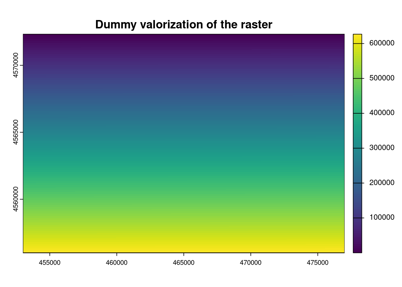
5.6 Raster drivers / formats
Here follows the list of drivers that are available in the current GDAL installation:
tab = terra::gdal(drivers = TRUE)| name | raster | vector | can | vsi | long.name |
|---|---|---|---|---|---|
| AAIGrid | TRUE | FALSE | read/write | TRUE | Arc/Info ASCII Grid |
| ACE2 | TRUE | FALSE | read | TRUE | ACE2 |
| ADRG | TRUE | FALSE | read/write | TRUE | ARC Digitized Raster Graphics |
| AIG | TRUE | FALSE | read | TRUE | Arc/Info Binary Grid |
| AirSAR | TRUE | FALSE | read | TRUE | AirSAR Polarimetric Image |
| AmigoCloud | FALSE | TRUE | read/write | FALSE | AmigoCloud |
| ARG | TRUE | FALSE | read/write | TRUE | Azavea Raster Grid format |
| AVCBin | FALSE | TRUE | read | TRUE | Arc/Info Binary Coverage |
| AVCE00 | FALSE | TRUE | read | TRUE | Arc/Info E00 (ASCII) Coverage |
| BAG | TRUE | TRUE | read/write | TRUE | Bathymetry Attributed Grid |
| BIGGIF | TRUE | FALSE | read | TRUE | Graphics Interchange Format (.gif) |
| BLX | TRUE | FALSE | read/write | TRUE | Magellan topo (.blx) |
| BMP | TRUE | FALSE | read/write | TRUE | MS Windows Device Independent Bitmap |
| BSB | TRUE | FALSE | read | TRUE | Maptech BSB Nautical Charts |
| BT | TRUE | FALSE | read/write | TRUE | VTP .bt (Binary Terrain) 1.3 Format |
| BYN | TRUE | FALSE | read/write | TRUE | Natural Resources Canada’s Geoid |
| CAD | TRUE | TRUE | read | TRUE | AutoCAD Driver |
| CALS | TRUE | FALSE | read/write | TRUE | CALS (Type 1) |
| Carto | FALSE | TRUE | read/write | FALSE | Carto |
| CEOS | TRUE | FALSE | read | TRUE | CEOS Image |
| COASP | TRUE | FALSE | read | FALSE | DRDC COASP SAR Processor Raster |
| COG | TRUE | FALSE | read/write | TRUE | Cloud optimized GeoTIFF generator |
| COSAR | TRUE | FALSE | read | TRUE | COSAR Annotated Binary Matrix (TerraSAR-X) |
| CPG | TRUE | FALSE | read | TRUE | Convair PolGASP |
| CSV | FALSE | TRUE | read/write | TRUE | Comma Separated Value (.csv) |
| CSW | FALSE | TRUE | read | FALSE | OGC CSW (Catalog Service for the Web) |
| CTable2 | TRUE | FALSE | read/write | TRUE | CTable2 Datum Grid Shift |
| CTG | TRUE | FALSE | read | TRUE | USGS LULC Composite Theme Grid |
| DAAS | TRUE | FALSE | read | FALSE | Airbus DS Intelligence Data As A Service driver |
| DERIVED | TRUE | FALSE | read | FALSE | Derived datasets using VRT pixel functions |
| DGN | FALSE | TRUE | read/write | TRUE | Microstation DGN |
| DIMAP | TRUE | FALSE | read | TRUE | SPOT DIMAP |
| DIPEx | TRUE | FALSE | read | TRUE | DIPEx |
| DOQ1 | TRUE | FALSE | read | TRUE | USGS DOQ (Old Style) |
| DOQ2 | TRUE | FALSE | read | TRUE | USGS DOQ (New Style) |
| DTED | TRUE | FALSE | read/write | TRUE | DTED Elevation Raster |
| DXF | FALSE | TRUE | read/write | TRUE | AutoCAD DXF |
| ECRGTOC | TRUE | FALSE | read | TRUE | ECRG TOC format |
| EDIGEO | FALSE | TRUE | read | TRUE | French EDIGEO exchange format |
| EEDA | FALSE | TRUE | read | FALSE | Earth Engine Data API |
| EEDAI | TRUE | FALSE | read | FALSE | Earth Engine Data API Image |
| EHdr | TRUE | FALSE | read/write | TRUE | ESRI .hdr Labelled |
| EIR | TRUE | FALSE | read | TRUE | Erdas Imagine Raw |
| ELAS | TRUE | FALSE | read/write | TRUE | ELAS |
| Elasticsearch | FALSE | TRUE | read/write | FALSE | Elastic Search |
| ENVI | TRUE | FALSE | read/write | TRUE | ENVI .hdr Labelled |
| ERS | TRUE | FALSE | read/write | TRUE | ERMapper .ers Labelled |
| ESAT | TRUE | FALSE | read | TRUE | Envisat Image Format |
| ESRI Shapefile | FALSE | TRUE | read/write | TRUE | ESRI Shapefile |
| ESRIC | TRUE | FALSE | read | TRUE | Esri Compact Cache |
| ESRIJSON | FALSE | TRUE | read | TRUE | ESRIJSON |
| FAST | TRUE | FALSE | read | TRUE | EOSAT FAST Format |
| FIT | TRUE | FALSE | read/write | TRUE | FIT Image |
| FITS | TRUE | TRUE | read/write | FALSE | Flexible Image Transport System |
| FlatGeobuf | FALSE | TRUE | read/write | TRUE | FlatGeobuf |
| GenBin | TRUE | FALSE | read | TRUE | Generic Binary (.hdr Labelled) |
| Geoconcept | FALSE | TRUE | read/write | TRUE | Geoconcept |
| GeoJSON | FALSE | TRUE | read/write | TRUE | GeoJSON |
| GeoJSONSeq | FALSE | TRUE | read/write | TRUE | GeoJSON Sequence |
| GeoRSS | FALSE | TRUE | read/write | TRUE | GeoRSS |
| GFF | TRUE | FALSE | read | TRUE | Ground-based SAR Applications Testbed File Format (.gff) |
| GIF | TRUE | FALSE | read/write | TRUE | Graphics Interchange Format (.gif) |
| GML | FALSE | TRUE | read/write | TRUE | Geography Markup Language (GML) |
| GMLAS | FALSE | TRUE | read/write | TRUE | Geography Markup Language (GML) driven by application schemas |
| GNMDatabase | FALSE | FALSE | read/write | FALSE | Geographic Network generic DB based model |
| GNMFile | FALSE | FALSE | read/write | FALSE | Geographic Network generic file based model |
| GPKG | TRUE | TRUE | read/write | TRUE | GeoPackage |
| GPSBabel | FALSE | TRUE | read/write | FALSE | GPSBabel |
| GPX | FALSE | TRUE | read/write | TRUE | GPX |
| GRASSASCIIGrid | TRUE | FALSE | read | TRUE | GRASS ASCII Grid |
| GRIB | TRUE | FALSE | read/write | TRUE | GRIdded Binary (.grb, .grb2) |
| GS7BG | TRUE | FALSE | read/write | TRUE | Golden Software 7 Binary Grid (.grd) |
| GSAG | TRUE | FALSE | read/write | TRUE | Golden Software ASCII Grid (.grd) |
| GSBG | TRUE | FALSE | read/write | TRUE | Golden Software Binary Grid (.grd) |
| GSC | TRUE | FALSE | read | TRUE | GSC Geogrid |
| GTFS | FALSE | TRUE | read | TRUE | General Transit Feed Specification |
| GTiff | TRUE | FALSE | read/write | TRUE | GeoTIFF |
| GTX | TRUE | FALSE | read/write | TRUE | NOAA Vertical Datum .GTX |
| GXF | TRUE | FALSE | read | TRUE | GeoSoft Grid Exchange Format |
| HDF4 | TRUE | FALSE | read | FALSE | Hierarchical Data Format Release 4 |
| HDF4Image | TRUE | FALSE | read/write | FALSE | HDF4 Dataset |
| HDF5 | TRUE | FALSE | read | TRUE | Hierarchical Data Format Release 5 |
| HDF5Image | TRUE | FALSE | read | TRUE | HDF5 Dataset |
| HEIF | TRUE | FALSE | read | TRUE | ISO/IEC 23008-12:2017 High Efficiency Image File Format |
| HF2 | TRUE | FALSE | read/write | TRUE | HF2/HFZ heightfield raster |
| HFA | TRUE | FALSE | read/write | TRUE | Erdas Imagine Images (.img) |
| HTTP | TRUE | TRUE | read | FALSE | HTTP Fetching Wrapper |
| Idrisi | FALSE | TRUE | read | TRUE | Idrisi Vector (.vct) |
| ILWIS | TRUE | FALSE | read/write | TRUE | ILWIS Raster Map |
| Interlis 1 | FALSE | TRUE | read/write | TRUE | Interlis 1 |
| Interlis 2 | FALSE | TRUE | read/write | TRUE | Interlis 2 |
| IRIS | TRUE | FALSE | read | TRUE | IRIS data (.PPI, .CAPPi etc) |
| ISCE | TRUE | FALSE | read/write | TRUE | ISCE raster |
| ISG | TRUE | FALSE | read | TRUE | International Service for the Geoid |
| ISIS2 | TRUE | FALSE | read/write | TRUE | USGS Astrogeology ISIS cube (Version 2) |
| ISIS3 | TRUE | FALSE | read/write | TRUE | USGS Astrogeology ISIS cube (Version 3) |
| JAXAPALSAR | TRUE | FALSE | read | TRUE | JAXA PALSAR Product Reader (Level 1.1/1.5) |
| JDEM | TRUE | FALSE | read | TRUE | Japanese DEM (.mem) |
| JML | FALSE | TRUE | read/write | TRUE | OpenJUMP JML |
| JP2OpenJPEG | TRUE | TRUE | read/write | TRUE | JPEG-2000 driver based on OpenJPEG library |
| JPEG | TRUE | FALSE | read/write | TRUE | JPEG JFIF |
| JSONFG | FALSE | TRUE | read/write | TRUE | OGC Features and Geometries JSON |
| KML | FALSE | TRUE | read/write | TRUE | Keyhole Markup Language (KML) |
| KMLSUPEROVERLAY | TRUE | FALSE | read/write | TRUE | Kml Super Overlay |
| KRO | TRUE | FALSE | read/write | TRUE | KOLOR Raw |
| L1B | TRUE | FALSE | read | TRUE | NOAA Polar Orbiter Level 1b Data Set |
| LAN | TRUE | FALSE | read/write | TRUE | Erdas .LAN/.GIS |
| LCP | TRUE | FALSE | read/write | TRUE | FARSITE v.4 Landscape File (.lcp) |
| Leveller | TRUE | FALSE | read/write | TRUE | Leveller heightfield |
| LIBKML | FALSE | TRUE | read/write | TRUE | Keyhole Markup Language (LIBKML) |
| LOSLAS | TRUE | FALSE | read | TRUE | NADCON .los/.las Datum Grid Shift |
| LVBAG | FALSE | TRUE | read | TRUE | Kadaster LV BAG Extract 2.0 |
| MAP | TRUE | FALSE | read | TRUE | OziExplorer .MAP |
| MapInfo File | FALSE | TRUE | read/write | TRUE | MapInfo File |
| MapML | FALSE | TRUE | read/write | TRUE | MapML |
| MBTiles | TRUE | TRUE | read/write | TRUE | MBTiles |
| MEM | TRUE | FALSE | read/write | FALSE | In Memory Raster |
| Memory | FALSE | TRUE | read/write | FALSE | Memory |
| MFF | TRUE | FALSE | read/write | TRUE | Vexcel MFF Raster |
| MFF2 | TRUE | FALSE | read/write | FALSE | Vexcel MFF2 (HKV) Raster |
| MRF | TRUE | FALSE | read/write | TRUE | Meta Raster Format |
| MSGN | TRUE | FALSE | read | TRUE | EUMETSAT Archive native (.nat) |
| MSSQLSpatial | FALSE | TRUE | read/write | FALSE | Microsoft SQL Server Spatial Database |
| MVT | FALSE | TRUE | read/write | TRUE | Mapbox Vector Tiles |
| MySQL | FALSE | TRUE | read/write | FALSE | MySQL |
| NAS | FALSE | TRUE | read | TRUE | NAS - ALKIS |
| NDF | TRUE | FALSE | read | TRUE | NLAPS Data Format |
| netCDF | TRUE | TRUE | read/write | FALSE | Network Common Data Format |
| NGSGEOID | TRUE | FALSE | read | TRUE | NOAA NGS Geoid Height Grids |
| NGW | TRUE | TRUE | read/write | FALSE | NextGIS Web |
| NITF | TRUE | FALSE | read/write | TRUE | National Imagery Transmission Format |
| NOAA_B | TRUE | FALSE | read | TRUE | NOAA GEOCON/NADCON5 .b format |
| NSIDCbin | TRUE | FALSE | read | TRUE | NSIDC Sea Ice Concentrations binary (.bin) |
| NTv2 | TRUE | FALSE | read/write | TRUE | NTv2 Datum Grid Shift |
| NWT_GRC | TRUE | FALSE | read | TRUE | Northwood Classified Grid Format .grc/.tab |
| NWT_GRD | TRUE | FALSE | read/write | TRUE | Northwood Numeric Grid Format .grd/.tab |
| OAPIF | FALSE | TRUE | read | FALSE | OGC API - Features |
| ODBC | FALSE | TRUE | read | FALSE | |
| ODS | FALSE | TRUE | read/write | TRUE | Open Document/ LibreOffice / OpenOffice Spreadsheet |
| OGCAPI | TRUE | TRUE | read | TRUE | OGCAPI |
| OGR_GMT | FALSE | TRUE | read/write | TRUE | GMT ASCII Vectors (.gmt) |
| OGR_OGDI | FALSE | TRUE | read | FALSE | OGDI Vectors (VPF, VMAP, DCW) |
| OGR_PDS | FALSE | TRUE | read | TRUE | Planetary Data Systems TABLE |
| OGR_SDTS | FALSE | TRUE | read | TRUE | SDTS |
| OGR_VRT | FALSE | TRUE | read | TRUE | VRT - Virtual Datasource |
| OpenFileGDB | TRUE | TRUE | read/write | TRUE | ESRI FileGDB |
| OSM | FALSE | TRUE | read | TRUE | OpenStreetMap XML and PBF |
| OZI | TRUE | FALSE | read | TRUE | OziExplorer Image File |
| PAux | TRUE | FALSE | read/write | TRUE | PCI .aux Labelled |
| PCIDSK | TRUE | TRUE | read/write | TRUE | PCIDSK Database File |
| PCRaster | TRUE | FALSE | read/write | FALSE | PCRaster Raster File |
| TRUE | TRUE | read/write | TRUE | Geospatial PDF | |
| PDS | TRUE | FALSE | read | TRUE | NASA Planetary Data System |
| PDS4 | TRUE | TRUE | read/write | TRUE | NASA Planetary Data System 4 |
| PGDUMP | FALSE | TRUE | read/write | TRUE | PostgreSQL SQL dump |
| PGeo | FALSE | TRUE | read | FALSE | ESRI Personal GeoDatabase |
| PLMOSAIC | TRUE | FALSE | read | FALSE | Planet Labs Mosaics API |
| PLSCENES | TRUE | TRUE | read | FALSE | Planet Labs Scenes API |
| PMTiles | FALSE | TRUE | read/write | TRUE | ProtoMap Tiles |
| PNG | TRUE | FALSE | read/write | TRUE | Portable Network Graphics |
| PNM | TRUE | FALSE | read/write | TRUE | Portable Pixmap Format (netpbm) |
| PostGISRaster | TRUE | FALSE | read/write | FALSE | PostGIS Raster driver |
| PostgreSQL | FALSE | TRUE | read/write | FALSE | PostgreSQL/PostGIS |
| PRF | TRUE | FALSE | read | TRUE | Racurs PHOTOMOD PRF |
| R | TRUE | FALSE | read/write | TRUE | R Object Data Store |
| Rasterlite | TRUE | FALSE | read/write | TRUE | Rasterlite |
| RIK | TRUE | FALSE | read | TRUE | Swedish Grid RIK (.rik) |
| RMF | TRUE | FALSE | read/write | TRUE | Raster Matrix Format |
| ROI_PAC | TRUE | FALSE | read/write | TRUE | ROI_PAC raster |
| RPFTOC | TRUE | FALSE | read | TRUE | Raster Product Format TOC format |
| RRASTER | TRUE | FALSE | read/write | TRUE | R Raster |
| RS2 | TRUE | FALSE | read | TRUE | RadarSat 2 XML Product |
| RST | TRUE | FALSE | read/write | TRUE | Idrisi Raster A.1 |
| S102 | TRUE | FALSE | read | TRUE | S-102 Bathymetric Surface Product |
| S57 | FALSE | TRUE | read/write | TRUE | IHO S-57 (ENC) |
| SAFE | TRUE | FALSE | read | TRUE | Sentinel-1 SAR SAFE Product |
| SAGA | TRUE | FALSE | read/write | TRUE | SAGA GIS Binary Grid (.sdat, .sg-grd-z) |
| SAR_CEOS | TRUE | FALSE | read | TRUE | CEOS SAR Image |
| SDTS | TRUE | FALSE | read | TRUE | SDTS Raster |
| Selafin | FALSE | TRUE | read/write | TRUE | Selafin |
| SENTINEL2 | TRUE | FALSE | read | TRUE | Sentinel 2 |
| SGI | TRUE | FALSE | read/write | TRUE | SGI Image File Format 1.0 |
| SIGDEM | TRUE | FALSE | read/write | TRUE | Scaled Integer Gridded DEM .sigdem |
| SNODAS | TRUE | FALSE | read | TRUE | Snow Data Assimilation System |
| SOSI | FALSE | TRUE | read | FALSE | Norwegian SOSI Standard |
| SQLite | FALSE | TRUE | read/write | TRUE | SQLite / Spatialite |
| SRP | TRUE | FALSE | read | TRUE | Standard Raster Product (ASRP/USRP) |
| SRTMHGT | TRUE | FALSE | read/write | TRUE | SRTMHGT File Format |
| STACIT | TRUE | FALSE | read | TRUE | Spatio-Temporal Asset Catalog Items |
| STACTA | TRUE | FALSE | read | TRUE | Spatio-Temporal Asset Catalog Tiled Assets |
| SVG | FALSE | TRUE | read | TRUE | Scalable Vector Graphics |
| SXF | FALSE | TRUE | read | TRUE | Storage and eXchange Format |
| Terragen | TRUE | FALSE | read/write | TRUE | Terragen heightfield |
| TGA | TRUE | FALSE | read | TRUE | TGA/TARGA Image File Format |
| TIGER | FALSE | TRUE | read | TRUE | U.S. Census TIGER/Line |
| TIL | TRUE | FALSE | read | TRUE | EarthWatch .TIL |
| TopoJSON | FALSE | TRUE | read | TRUE | TopoJSON |
| TSX | TRUE | FALSE | read | TRUE | TerraSAR-X Product |
| UK .NTF | FALSE | TRUE | read | TRUE | UK .NTF |
| USGSDEM | TRUE | FALSE | read/write | TRUE | USGS Optional ASCII DEM (and CDED) |
| VDV | FALSE | TRUE | read/write | TRUE | VDV-451/VDV-452/INTREST Data Format |
| VFK | FALSE | TRUE | read | FALSE | Czech Cadastral Exchange Data Format |
| VICAR | TRUE | TRUE | read/write | TRUE | MIPL VICAR file |
| VRT | TRUE | FALSE | read/write | TRUE | Virtual Raster |
| WAsP | FALSE | TRUE | read/write | TRUE | WAsP .map format |
| WCS | TRUE | FALSE | read | TRUE | OGC Web Coverage Service |
| WEBP | TRUE | FALSE | read/write | TRUE | WEBP |
| WFS | FALSE | TRUE | read | TRUE | OGC WFS (Web Feature Service) |
| WMS | TRUE | FALSE | read/write | TRUE | OGC Web Map Service |
| WMTS | TRUE | FALSE | read/write | TRUE | OGC Web Map Tile Service |
| XLS | FALSE | TRUE | read | FALSE | MS Excel format |
| XLSX | FALSE | TRUE | read/write | TRUE | MS Office Open XML spreadsheet |
| XPM | TRUE | FALSE | read/write | TRUE | X11 PixMap Format |
| XYZ | TRUE | FALSE | read/write | TRUE | ASCII Gridded XYZ |
| Zarr | TRUE | FALSE | read/write | TRUE | Zarr |
| ZMap | TRUE | FALSE | read/write | TRUE | ZMap Plus Grid |
5.7 Export raster
terra::writeRaster( GRID, "DummyRaster.tif", overwrite=TRUE )5.8 Remote Sensing: R fundamentals
This part provides a basic overview about how to work with remote sensing data in R.
5.8.1 MODIS
The Moderate Resolution Imaging Spectroradiometer (MODIS) is an optical sensor onboard two satellites named Terra (originally known as EOS AM-1) and Aqua (originally known as EOS PM-1) operated by NASA. Terra was launched on 18 December 1999 and Aqua was launched on 24 May 2002. Terra’s orbit around the Earth is such that it passes from North to South across the equator in the morning, while Aqua passes South to North over the equator in the afternoon. Terra MODIS and Aqua MODIS take images for the entire Earth’s surface every 1 to 2 days. The data collected is the intensity of the light reflected by earth in 36 different wavelengths (“colors”). Both Terra and Aqua also have other sensors besides MODIS. These two sensors have publicly available daily archive of conditions on the earth surface for the past 20 years!
5.8.1.1 Data products
Data products are listed here: https://modis.gsfc.nasa.gov/data/dataprod/.
5.8.1.1.1 File Naming Convention
For example: MCD15A3H.A2025213.h11v06.061.2025218033608.hdf
The file name begins with the Product Short Name (e.g. MYD13Q1 for NDVI or MCD15A3H for LAI) followed by the Julian Date of Acquisition formatted as AYYYYDDD (e.g. A2025213), the Tile Identifier which is horizontal tile and vertical tile provided as hXXvYY (h11v06), the Version of the data collection (061), the Julian Date and Time of Production designated as YYYYDDDHHMMSS (2025218033608), and the Data Format (hdf).
5.8.1.2 Vegetation index products
MODIS vegetation indices, produced on 16-day intervals and at multiple spatial resolutions, provide consistent spatial and temporal comparisons of vegetation canopy greenness, a composite property of leaf area, chlorophyll and canopy structure. Two vegetation indices are derived from atmospherically-corrected reflectance in the red, near-infrared, and blue wavebands; the normalized difference vegetation index (NDVI), which provides continuity with NOAA’s AVHRR NDVI time series record for historical and climate applications, and the enhanced vegetation index (EVI), which minimizes canopy-soil variations and improves sensitivity over dense vegetation conditions. The two products more effectively characterize the global range of vegetation states and processes.
| Product Name | Terra | Aqua |
|---|---|---|
| Vegetation Indices 16-Day L3 Global 250m | MOD13Q1 | MYD13Q1 |
| Vegetation Indices 16-Day L3 Global 500m | MOD13A1 | MYD13A1 |
| Vegetation Indices 16-Day L3 Global 1km | MOD13A2 | MYD13A2 |
| Vegetation Indices 16-Day L3 Global 0.05Deg CMG | MOD13C1 | MYD13C1 |
| Vegetation Indices Monthly L3 Global 1km | MOD13A3 | MYD13A3 |
| Vegetation Indices Monthly L3 Global 0.05Deg CMG | MOD13C2 | MYD13C2 |
5.8.1.3 R: download MODIS data
The MYD13Q1 Version 6 data product was decommissioned on July 31, 2023. Users are encouraged to use the **M*D13Q1 Version 6.1** data product.
Read this chapter to get an introduction about the MODIS data.
Terra Vegetation Indices:
getProducts("MOD13Q1")
#>          provider             concept_id short_name version
#> 71204     LPCLOUD    C2763375196-LPCLOUD    MOD13Q1     003
#> 106844 LPDAAC_ECS   C50878306-LPDAAC_ECS    MOD13Q1     003
#> 34745  LPDAAC_ECS   C16893882-LPDAAC_ECS    MOD13Q1     004
#> 71042     LPCLOUD    C2763372101-LPCLOUD    MOD13Q1     004
#> 3166   LPDAAC_ECS  C107705237-LPDAAC_ECS    MOD13Q1     005
#> 70376     LPCLOUD    C2763272859-LPCLOUD    MOD13Q1     005
#> 39914  LPDAAC_ECS  C194001241-LPDAAC_ECS    MOD13Q1     006
#> 70785     LPCLOUD    C2763298064-LPCLOUD    MOD13Q1     006
#> 96862     LPCLOUD    C3675550934-LPCLOUD    MOD13Q1     007
#> 30009  LPDAAC_ECS C1621383370-LPDAAC_ECS    MOD13Q1     061
#> 36014     LPCLOUD    C1748066515-LPCLOUD    MOD13Q1     061
Aqua Vegetation Indices:
getProducts('MYD13Q1')
#>         provider             concept_id short_name version
#> 71141    LPCLOUD    C2763373539-LPCLOUD    MYD13Q1     004
#> 80935 LPDAAC_ECS   C28901529-LPDAAC_ECS    MYD13Q1     004
#> 3439  LPDAAC_ECS  C115315503-LPDAAC_ECS    MYD13Q1     005
#> 70447    LPCLOUD    C2763279070-LPCLOUD    MYD13Q1     005
#> 39881 LPDAAC_ECS  C194001221-LPDAAC_ECS    MYD13Q1     006
#> 70910    LPCLOUD    C2763370237-LPCLOUD    MYD13Q1     006
#> 96865    LPCLOUD    C3675551131-LPCLOUD    MYD13Q1     007
#> 30108 LPDAAC_ECS C1621431683-LPDAAC_ECS    MYD13Q1     061
#> 55311    LPCLOUD    C2307290656-LPCLOUD    MYD13Q1     061
This points to the decommissioned version 6:
productInfo("MYD13Q1")Select Belgium as Area of Interest (AoI):
library(geobounds)
bel <- gb_get_adm0("BEL")
Plot Belgium admin bourders:
library(tmap)
tmap_mode("view")
tm_shape(bel) + tm_borders(col="gray50",lwd=3)
Check images:
f <- getNASA( product="MOD13Q1", version = '061',
              start_date = "2026-01-01", end_date = "2026-03-31",
              aoi = bel,
              download = FALSE)
This command returns temporal details about the found tiles:
modisDate(f)| Product | Julian day | Date | Tile | File name |
|---|---|---|---|---|
| MOD13Q1 | A2025353 | 2025-12-19 | h18v03 | MOD13Q1.A2025353.h18v03.061.2026005201731.hdf |
| MOD13Q1 | A2025353 | 2025-12-19 | h18v04 | MOD13Q1.A2025353.h18v04.061.2026005202746.hdf |
| MOD13Q1 | A2026001 | 2026-01-01 | h18v04 | MOD13Q1.A2026001.h18v04.061.2026019192521.hdf |
| MOD13Q1 | A2026001 | 2026-01-01 | h18v03 | MOD13Q1.A2026001.h18v03.061.2026019192439.hdf |
| MOD13Q1 | A2026017 | 2026-01-17 | h18v03 | MOD13Q1.A2026017.h18v03.061.2026034010243.hdf |
| MOD13Q1 | A2026017 | 2026-01-17 | h18v04 | MOD13Q1.A2026017.h18v04.061.2026034010157.hdf |
| MOD13Q1 | A2026033 | 2026-02-02 | h18v04 | MOD13Q1.A2026033.h18v04.061.2026051102017.hdf |
| MOD13Q1 | A2026033 | 2026-02-02 | h18v03 | MOD13Q1.A2026033.h18v03.061.2026051101003.hdf |
| MOD13Q1 | A2026049 | 2026-02-18 | h18v03 | MOD13Q1.A2026049.h18v03.061.2026071114845.hdf |
| MOD13Q1 | A2026049 | 2026-02-18 | h18v04 | MOD13Q1.A2026049.h18v04.061.2026071114856.hdf |
| MOD13Q1 | A2026065 | 2026-03-06 | h18v03 | MOD13Q1.A2026065.h18v03.061.2026083115010.hdf |
| MOD13Q1 | A2026065 | 2026-03-06 | h18v04 | MOD13Q1.A2026065.h18v04.061.2026083115121.hdf |
| MOD13Q1 | A2026081 | 2026-03-22 | h18v04 | MOD13Q1.A2026081.h18v04.061.2026098000619.hdf |
| MOD13Q1 | A2026081 | 2026-03-22 | h18v03 | MOD13Q1.A2026081.h18v03.061.2026098000852.hdf |
I cannot share my username and password but you can register at https://urs.earthdata.nasa.gov/users/new:
usr = "..."
pwd = "..."
Actually get the images:
f <- getNASA( product="MOD13Q1", version = '061',
              username = usr, password = pwd,
              start_date = "2026-03-06", end_date = "2026-03-06",
              aoi = bel,
              download = TRUE,
              path = '/home/giuliano/datasets/rMODIS/')
Read MODIS Aqua (MOD13Q1) tiles (h18v03 and h18v04) over Belgium on 06 March 2026 (A2026065):
mod13q1_1803 <- rast("MOD13Q1.A2026065.h18v03.061.2026083115010.hdf")
mod13q1_1804 <- rast("MOD13Q1.A2026065.h18v04.061.2026083115121.hdf")
Print raster metadata:
print(mod13q1_1803)
#> class       : SpatRaster
#> dimensions  : 4800, 4800, 12  (nrow, ncol, nlyr)
#> resolution  : 231.6564, 231.6564  (x, y)
#> extent      : 0, 1111951, 5559753, 6671703  (xmin, xmax, ymin, ymax)
#> coord. ref. : +proj=sinu +lon_0=0 +x_0=0 +y_0=0 +R=6371007.181 +units=m +no_defs
#> sources     : MOD13Q1.A2026065.h18v03.061.2026083115010.hdf:MODIS_Grid_16DAY_250m_500m_VI:250m 16 days NDVI
#>               MOD13Q1.A2026065.h18v03.061.2026083115010.hdf:MODIS_Grid_16DAY_250m_500m_VI:250m 16 days EVI
#>               MOD13Q1.A2026065.h18v03.061.2026083115010.hdf:MODIS_Grid_16DAY_250m_500m_VI:250m 16 days VI Quality
#>               ... and 9 more sources
#> varnames    : MOD13Q1.A2026065.h18v03.061.2026083115010
#>               MOD13Q1.A2026065.h18v03.061.2026083115010
#>               MOD13Q1.A2026065.h18v03.061.2026083115010
#>               ...
#> names       : "250m~NDVI", "250m~ EVI", "250m~lity", "250m~ance", "250m~ance", "250m~ance", ...
Check that they have the same CRS:
Crop the two multi-band rasters for Belgium:
bel_proj <- st_transform(bel, st_crs(mod13q1_1803))

bel_1803 <- crop(mod13q1_1803,bel_proj)
bel_1804 <- crop(mod13q1_1804,bel_proj)

plot(bel_1803)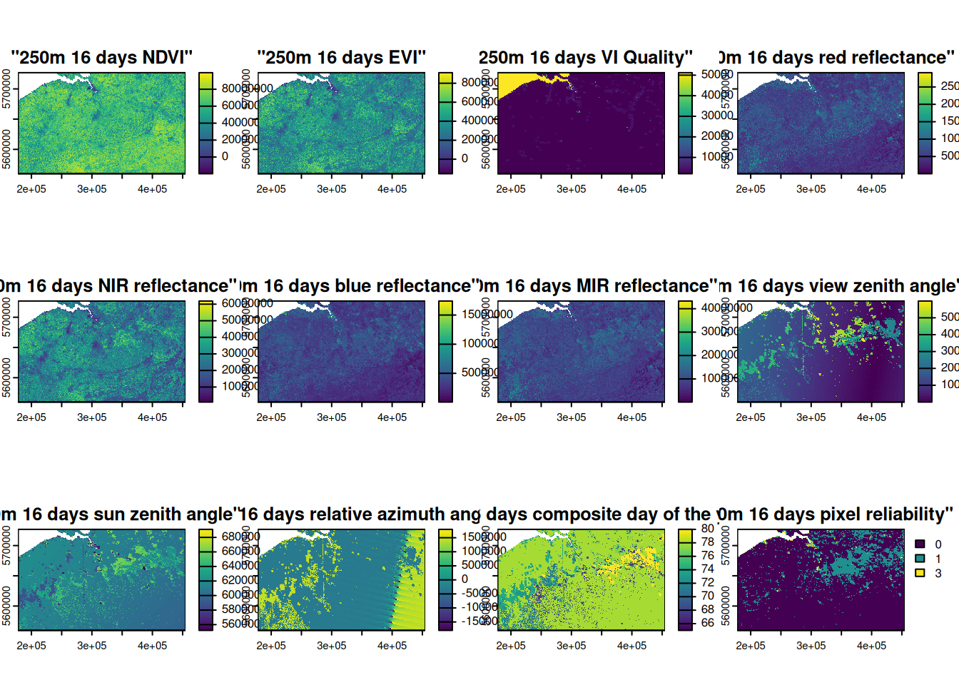
Merge the two tiles covering Belgium:
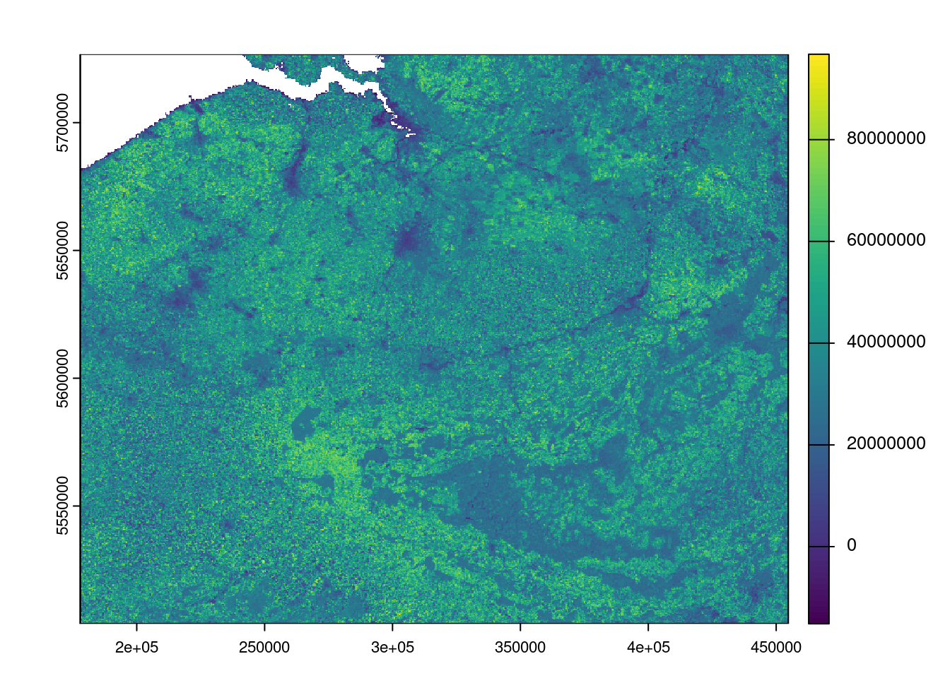
Select EVI band:
bel_evi <- bel_mod13q1$`"250m 16 days EVI"`
bel_evi
#> class       : SpatRaster
#> dimensions  : 962, 1195, 1  (nrow, ncol, nlyr)
#> resolution  : 231.6564, 231.6564  (x, y)
#> extent      : 177912.1, 454741.4, 5503923, 5726777  (xmin, xmax, ymin, ymax)
#> coord. ref. : +proj=sinu +lon_0=0 +x_0=0 +y_0=0 +R=6371007.181 +units=m +no_defs
#> source(s)   : memory
#> varname     : MOD13Q1.A2026065.h18v03.061.2026083115010
#> name        : "250m 16 days EVI"
#> min value   :          -15290000
#> max value   :           98910000
Plot
plot(bel_evi)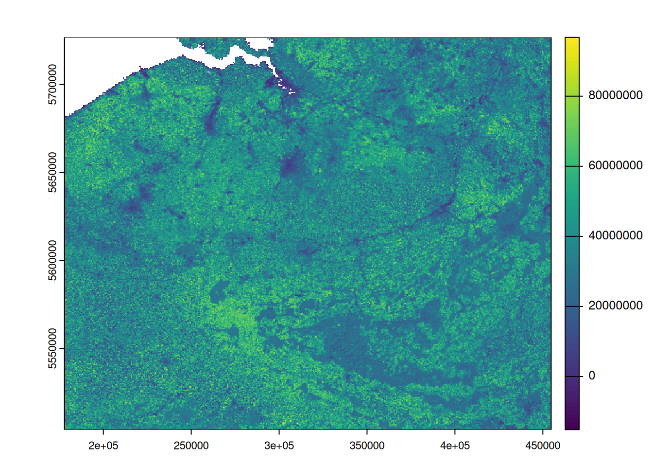
Crop for Belgium and mask pixels that are outside the AoI boundary as NA:
bel_evi_masked <- crop(bel_evi, bel_proj, mask=TRUE)EVI map for Belgium on 06 March 2026:
library(tmap)
tmap_mode("view")

tm_shape(bel_evi_masked) +
  tm_raster( col.scale = tm_scale_intervals(midpoint = NA) ) +
  tm_shape(bel_proj) + tm_borders(col="gray50",lwd=3)
5.8.2 Landsat 8/9 Operational Land Imager (OLI)
Read the Evolution of Landsat Spectral Bands to get more insights about evolution since 1970s. To maintain data continuity with earlier Landsat missions, Landsat 8 and 9 collect data in eight “heritage bands”: three visible bands, one near-infrared band, two shortwave-infrared bands, and two thermal-infrared bands. The Operational Land Imager (OLI) and Thermal Infrared Sensor (TIRS) instruments on Landsat 8 increased the total number of spectral bands to 11. On OLI, new bands included a coastal blue band (band 1) for ocean color observations in coastal zones and a shortwave-infrared band (band 9) which senses wavelengths that strongly absorb water vapor, allowing for the detection of cirrus clouds. The TIRS instrument collects data in two thermal bands (bands 10 and 11). These longer-wavelength bands play a vital role in measuring evapotranspiration to track water use, detect fire scars and volcanic lava flows, and calculate spectral indices to monitor land use.
| Band | Description | Wavelength_µm | GSD_m |
|---|---|---|---|
| B1 | Coastal / Aerosol | 0.43-0.45 | 30 |
| B2 | Blue | 0.45-0.51 | 30 |
| B3 | Green | 0.53-0.59 | 30 |
| B4 | Red | 0.64-0.67 | 30 |
| B5 | Near-infrared (NIR) | 0.85-0.88 | 30 |
| B6 | Shortwave-infrared (SWIR) 1 | 1.57-1.65 | 30 |
| B7 | Shortwave-infrared (SWIR) 2 | 2.11-2.29 | 30 |
| B8 | Panchromatic | 0.50-0.68 | 15 |
| B9 | Cirrus | 1.36-1.38 | 30 |
Add:
- Apply Landsat Collection 2 Level-2 scaling for Surface Reflectance –> explain how to rescale Surface Reflectance pixels according to the official documentation:
b <- b * 0.0000275 - 0.2 - QA layers and decode to filter for good quality pixels
5.9 Manipulate multidimensional raster data
5.9.1 Prepare multidimensional LAI dataset
Check the MODIS collection 6.1 LAI/FPAR Product User’s Guide for more information about the data used in this experiment.
Fundamental information is summirized here:| Information | Value |
|---|---|
| Available layers | Fpar_500m; Lai_500m; FparLai_QC; FparExtra_QC; FparStdDev_500m; LaiStdDev_500m |
| LAI data type | 8-bit unsigned integer |
| LAI scale factor | 0.1 |
| Example | 25 -> 2.5 LAI |
| Valid LAI range | 0-100 (equivalent to 0.0-10.0) |
| Fill / special values | 249-255 |
| QC data type | 8-bit unsigned integer (class flag) |
| QC recommendation | Use the QC layers to filter unreliable retrievals |
| Key QC field | SCF_QC |
| SCF_QC meaning | 000 main method; 001 saturation; 010/011 backup algorithm; 100 not produced |
| LaiStdDev_500m | Retrieval uncertainty, with scale factor 0.1 |
| Algorithm | Main LUT-based method + empirical backup based on NDVI |
5.9.1.1 AoI
Load required libraries:
Define the Area of Interest (AoI) in Calabria region in Italy:
it_regions = gb_get_adm2("ITA")
head(it_regions,n=2)
#> Simple feature collection with 2 features and 5 fields
#> Geometry type: MULTIPOLYGON
#> Dimension:     XY
#> Bounding box:  xmin: 6.626621 ymin: 44.06012 xmax: 9.21424 ymax: 46.46443
#> Geodetic CRS:  WGS 84
#> # A tibble: 2 × 6
#>   shapeName     shapeISO shapeID        shapeGroup shapeType
#>   <chr>         <chr>    <chr>          <chr>      <chr>
#> 1 Piemonte      <NA>     23120603B8325… ITA        ADM2
#> 2 Valle d'Aosta <NA>     23120603B4691… ITA        ADM2
#> # ℹ 1 more variable: geometry <MULTIPOLYGON [°]>
Select Calabria region:
cal <- it_regions |>
  filter(shapeName == 'Calabria') |>
  select(shapeName,geometry)

cal
#> Simple feature collection with 1 feature and 1 field
#> Geometry type: MULTIPOLYGON
#> Dimension:     XY
#> Bounding box:  xmin: 15.62969 ymin: 37.91575 xmax: 17.20653 ymax: 40.14393
#> Geodetic CRS:  WGS 84
#> # A tibble: 1 × 2
#>   shapeName                                         geometry
#>   <chr>                                   <MULTIPOLYGON [°]>
#> 1 Calabria  (((15.80144 39.70044, 15.80155 39.70037, 15.801…
Plot:
tmap_mode("plot")
tm_basemap("OpenStreetMap") +
  tm_shape(cal) + tm_borders(col="red", lwd=2)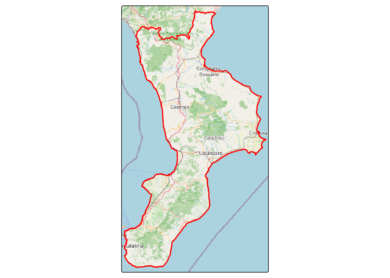
5.9.1.2 Select product
We select the 4-day 500m LAI with product name MCD15A3H according to the MODIS Leaf Area Index/FPAR web page. Version 6 is deprecated therefore we are interested in getting the MCD15A3H product version 6.1.
Search for LAI in MODIS in year 2025:
f <- getNASA( product='MCD15A3H', version = '061',
              start_date = "2025-01-01", end_date = "2025-12-31",
              aoi = cal,
              download = FALSE)
First 4 images:
head(f,n=4)
#> [1] "MCD15A3H.A2024361.h19v05.061.2025003200952.hdf"
#> [2] "MCD15A3H.A2024361.h19v04.061.2025003200959.hdf"
#> [3] "MCD15A3H.A2025001.h19v05.061.2025006155130.hdf"
#> [4] "MCD15A3H.A2025001.h19v04.061.2025006155140.hdf"
Last 4 images:
tail(f,n=4)
#> [1] "MCD15A3H.A2025361.h19v04.061.2026001034209.hdf"
#> [2] "MCD15A3H.A2025361.h19v05.061.2026001034256.hdf"
#> [3] "MCD15A3H.A2025365.h19v05.061.2026005233004.hdf"
#> [4] "MCD15A3H.A2025365.h19v04.061.2026005233730.hdf"
5.9.1.3 Get LAI images
Two tiles cover the Calabria region: h19v04 and h19v05, with {r} length(f) images for year 2025.
I cannot share my username and password but you can register at https://urs.earthdata.nasa.gov/users/new:
Download selected images:
f <- getNASA( product="MCD15A3H", version = '061',
              username = usr, password = pwd,
              start_date = "2025-01-01", end_date = "2025-12-31",
              aoi = cal,
              download = TRUE,
              path = '/home/giuliano/datasets/rMODIS/')
5.9.2 terra: LAI data
5.9.2.1 multi-dimensional LAI data
From the download before a LAI data cube was created:
lai25cal <- rast("/home/giuliano/datasets/rMODIS/LAI_2025_calabria.tif")
lai25cal
#> class       : SpatRaster
#> dimensions  : 500, 308, 92  (nrow, ncol, nlyr)
#> resolution  : 463.3127, 463.3127  (x, y)
#> extent      : 1343607, 1486307, 4216146, 4447802  (xmin, xmax, ymin, ymax)
#> coord. ref. : +proj=sinu +lon_0=0 +x_0=0 +y_0=0 +R=6371007.181 +units=m +no_defs
#> source      : LAI_2025_calabria.tif
#> names       : A2025001, A2025005, A2025009, A2025013, A2025017, A2025021, ...
#> min values  :      0.0,      0.0,      0.0,      0.0,      0.0,      0.0, ...
#> max values  :     25.4,     25.4,     25.4,     25.4,     25.4,     25.4, ...
We need to properly scale the LAI data using the 0.1 scale factor:
lai25cal <- lai25cal * 0.1Prepare the AoI in the same CRS of LAI:
cal_proj <- gb_get_adm2("ITA") |>
  filter(shapeName == 'Calabria') |>
  select(shapeName,geometry) |>
  st_transform(st_crs(lai25cal))
Map of LAI:
tmap_mode("plot")
tm_shape(lai25cal[[40]]) + tm_raster() +
  tm_shape(cal_proj) + tm_borders(col = "gray50", lwd=3)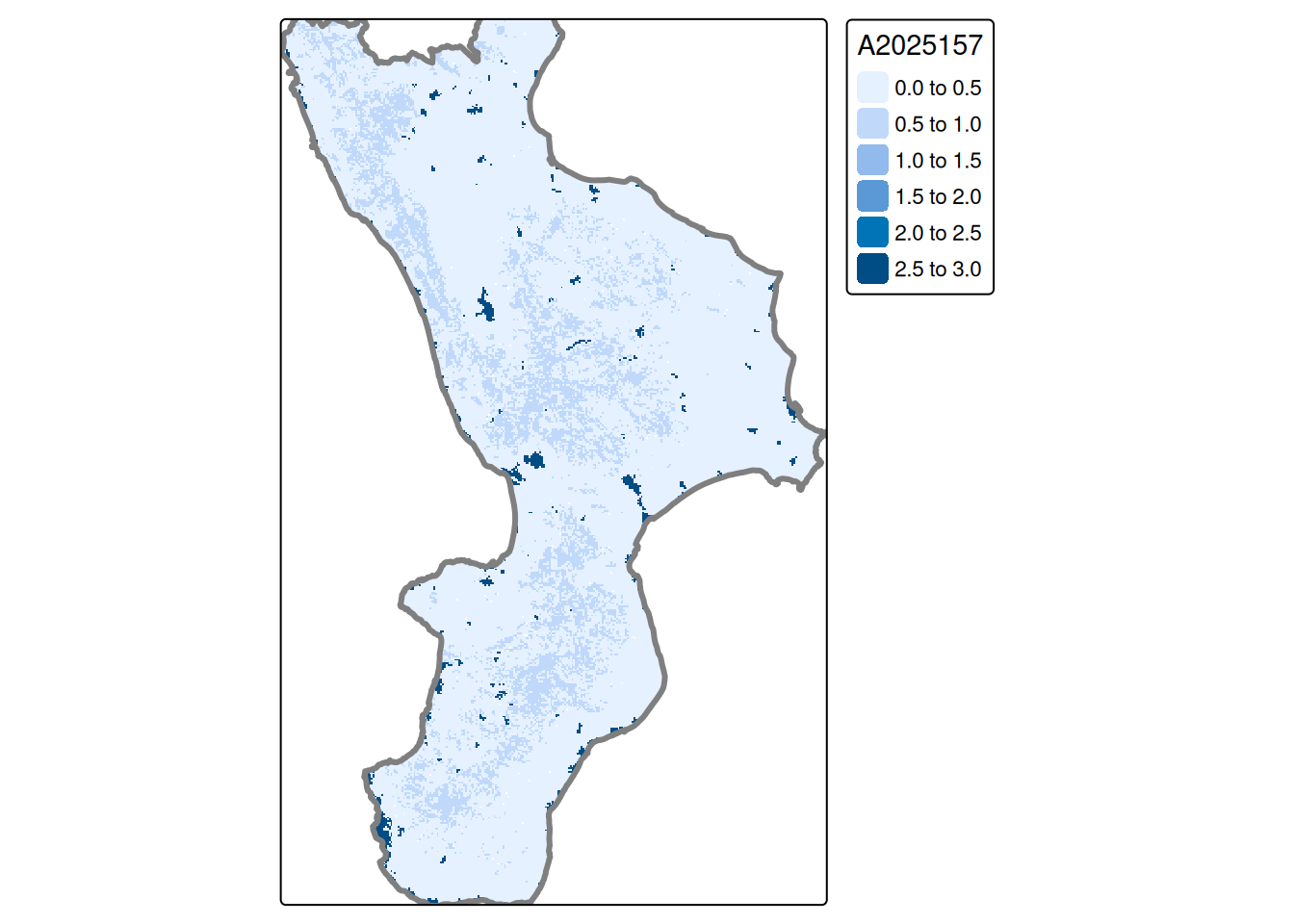
5.9.2.2 Random locations, for time-series analysis
Randomly select 50 points from Calabria administrative limit:
set.seed(1)
Pi <- st_sample( cal_proj,
                 size=50,
                 type='random',
                 exact=TRUE
               )

plot( cal_proj, col="gray80",
      main="Random locations", reset = FALSE )
points( Pi, pch = 16, col = "red" )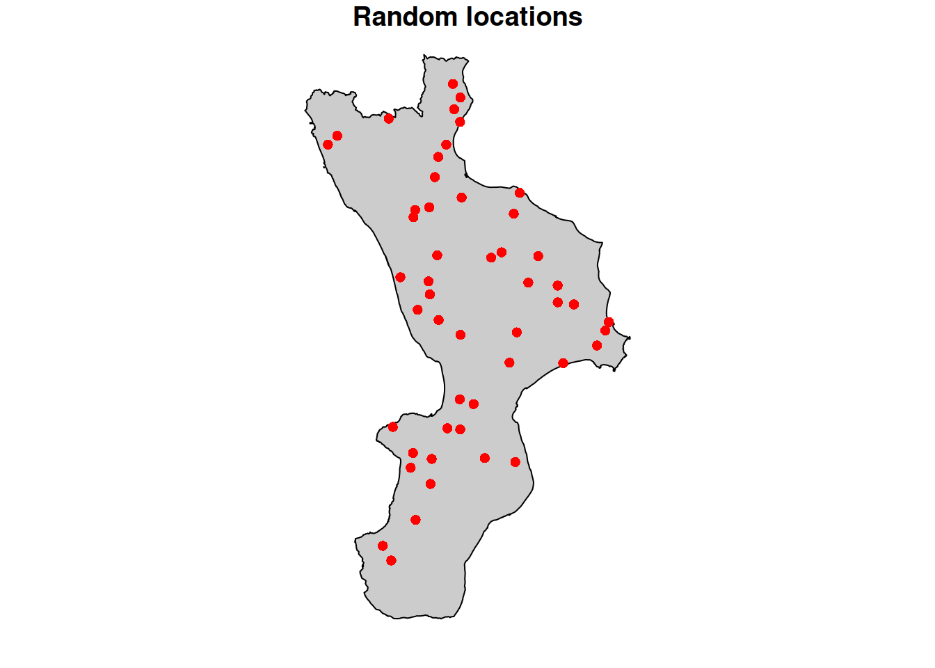
| Point | A2025001 | A2025005 | A2025009 | A2025013 | A2025017 | A2025021 |
|---|---|---|---|---|---|---|
| P_1 | 0.03 | 0.07 | 0.06 | 0.10 | 0.09 | 0.08 |
| P_2 | 0.02 | 0.06 | 0.06 | 0.01 | 0.11 | 0.11 |
| P_3 | 0.07 | 0.10 | 0.07 | 0.10 | 0.10 | 0.10 |
| P_4 | 0.16 | 0.13 | 0.15 | 0.00 | 0.07 | 0.18 |
| P_5 | 0.15 | 0.12 | 0.09 | 0.11 | 0.03 | 0.09 |
| P_6 | 0.19 | 0.10 | 0.10 | 0.19 | 0.00 | 0.10 |
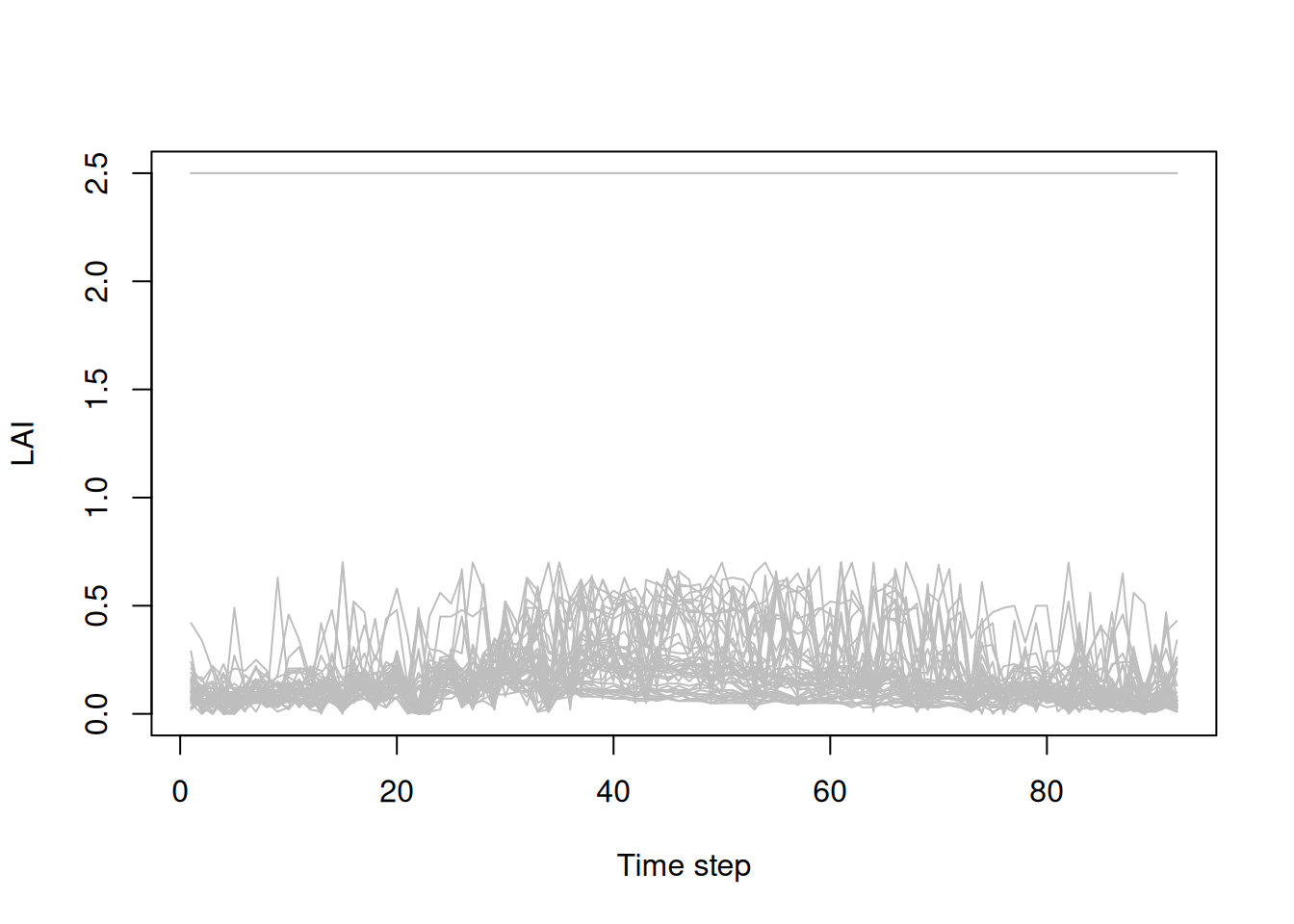
5.9.2.3 Charts for visual inspection
In the next charts we need to transpose the lai data.frame, because our variables are locations not dates:
Boxplot to detect distribution and anomalies.
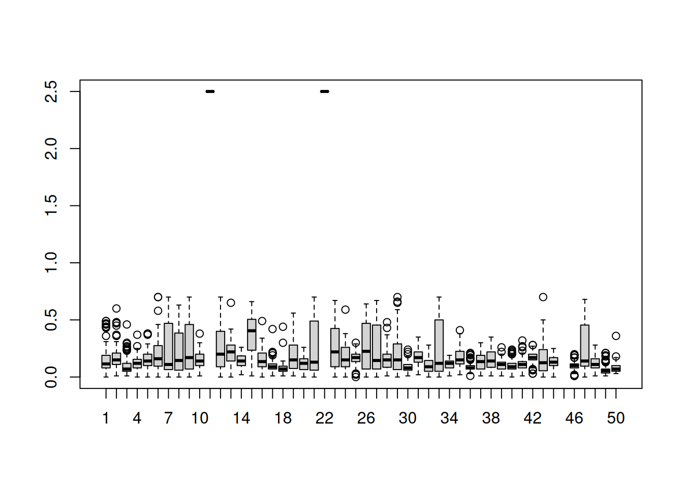
There are also anomalous and missing LAI values, as highlighted in the boxplot above:
5.9.2.4 Quality control
Missing values (NA) can be discarded while anomalous values must be investigated and removed from any analysis.
The FparLai_QC band in the original hdf file helps detecting anomalies enabling the user to skip bad values and retain only good ones.
5.9.2.4.1 Decoding the SCF_QC field from FparLai_QC
The FparLai_QC layer is stored as an 8-bit unsigned integer. This means that each pixel contains one integer value, but that value actually stores several pieces of quality information in its bits. In the official MOD15/MCD15 user guide, the SCF_QC field is identified as the key indicator of retrieval quality.
To extract SCF_QC, we read bits 5 to 7 from the integer value. In simple terms:
-
bitwShiftR(x, 5)moves the binary number 5 positions to the right -
bitwAnd(..., 7)keeps only the last 3 bits (7in binary is111)
So the decoding formula is:
scf_qc <- bitwAnd(bitwShiftR(qc_value, 5L), 7L)This converts the original QC integer into a small class code from 0 to 4.
5.9.2.4.2 SCF_QC classes
| SCF_QC | Meaning |
|---|---|
| 0 | Main method used, best result possible (no saturation) |
| 1 | Main method used with saturation, good and very usable |
| 2 | Main method failed because of bad geometry; empirical algorithm used |
| 3 | Main method failed for other reasons; empirical algorithm used |
| 4 | Pixel not produced / value could not be retrieved |
These class meanings come directly from the official MOD15/MCD15 user guide.
5.9.2.4.3 QC in our case study
Get the FparLai_QC band for the first Julian day in 2025:
qc <- "MCD15A3H.A2025001.h19v05.061.2025006155130.hdf" |>
  rast(lyrs="FparLai_QC")

#> class       : SpatRaster
#> dimensions  : 2400, 2400, 1  (nrow, ncol, nlyr)
#> resolution  : 463.3127, 463.3127  (x, y)
#> extent      : 1111951, 2223901, 3335852, 4447802  (xmin, xmax, ymin, ymax)
#> coord. ref. : +proj=sinu +lon_0=0 +x_0=0 +y_0=0 +R=6371007.181 +units=m +no_defs
#> source      : MCD15A3H.A2025001.h19v05.061.2025006155130.hdf:MOD_Grid_MCD15A3H:FparLai_QC
#> varname     : MCD15A3H.A2025001.h19v05.061.2025006155130
#> name        : FparLai_QC
Get FparLai_QC values (namely qci) at the randomly selected locations Pi:
qci <- qc |>
  extract( vect(Pi) ) |>
  select(FparLai_QC) |>
  unlist() |>
  as.integer()

print(qci)
#>  [1]   0  16   2   2   0   0   0   0   0   0 157   2   0   2
#> [15]  32   2   0   0   2   0   0 157   0   2   2  65   2   0
#> [29]   0   2   0  10   0   0   0   0   2   0   2   2   0   2
#> [43]   0   2  NA   2   0   2   0   0
Decode the FparLai_QC values to extract the SCF_QC flags according to the official documentation summarised before:
scf_qci <- bitwAnd(bitwShiftR(qci, 5), 7)
scf_qci
#>  [1]  0  0  0  0  0  0  0  0  0  0  4  0  0  0  1  0  0  0
#> [19]  0  0  0  4  0  0  0  2  0  0  0  0  0  0  0  0  0  0
#> [37]  0  0  0  0  0  0  0  0 NA  0  0  0  0  0
Check the LAI values compared with the QC flag:
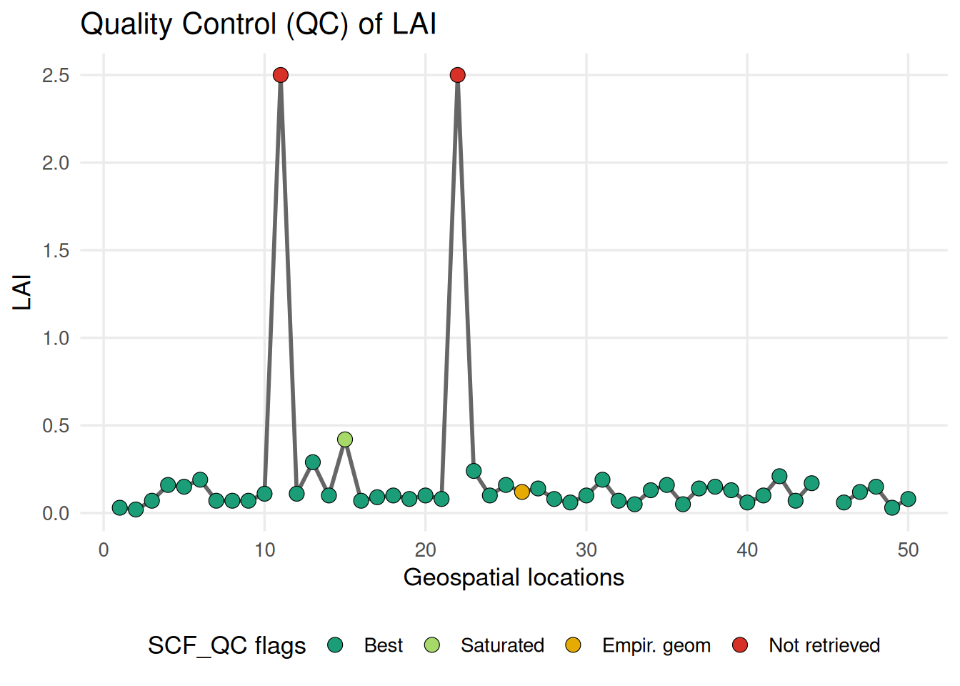
Most sampled points show consistent LAI values associated with good-quality retrievals, but a few cases remain unclear: some locations have a constant LAI value throughout the year (LAI=2.5) while their QC flag (=4, red marker) indicates that the pixel was not successfully retrieved. This apparent inconsistency deserves further investigation and highlights the importance of carefully checking product quality information in remote sensing analyses.