24 Exercises

24.1 Vector Geodata

24.1.1 Upper Secondary School

Objective: create a Simple Feature object in R to manage and represent (the position and other attributes of) your upper secondary school.
Folder: ‘didattica/assignments/vector_ex01/’

Use Google Maps to get the coordinates of your school and populate the following attributes:

geometry: POINT XY (2D)
CRS: 4326 (as used in Google)
attributes:
- ‘Name’
- ‘Surname’
- ‘SchoolName’
- ‘GraduationDate’

Note: do not change the labels used for the attributes, including lowercase / uppercase characters.

Deliver the file named name_surname_school.geojson in the folder ‘didattica/assignments/vector_ex01/’.
[E.g. giuliano_langella_school.geojson]

Once all students complete the previous step, in folder vector_ex01 there will be more files. Each student has to import in R all the files and create a unique SF object in R fusing all the vector data from all students.

24.1.2 Agraria Teaching Rooms

Objective: create a map with all Points of Interest (PoI) of the Dep. of Agriculture in Portici.
Folder: ‘didattica/assignments/vector_ex02/’
Source: Lecture and study rooms

Note: do not change the labels used for the attributes, including lowercase / uppercase characters.

24.1.2.1 Instructions

Each student select one or more PoIs within the Department (select different PoIs)
Go to geojson.io and draw a point on the map where you want to create a PoI
Add the following attributes (take care of the UPPERCASE / lowercase letters):
- ‘Aula’ → e.g. 1
- ‘Ubicazione’ → e.g. Mascabruno
- ‘Piano’ → e.g. Terra
- ‘Posti’ → e.g. 200
- ‘Descrizione’. → e.g. TAL
Export from geojson.io using format GeoJSON.
Load in RStudio Server file system
Import in R as Simple Feature
Create a plot / map to visualize the PoIs
Export the simple feature using filename such as name_surname_poistudent.geojson (e.g. giuliano_langella_poistudent.geojson) in the shared folder ’didattica/assignments/vector_ex02/
Wait that all students save their file
Load in R all the files and create a unique SF object in R fusing all the PoIs from all students
Save the SF object with all PoIs as name_surname_poiagraria.geojson (e.g. giuliano_langella_poiagraria.geojson)

24.1.3 Monumental trees

Objective: Create a simple feature of monumental trees in Italy.
Folder: ‘didattica/assignments/vector_ex03/’

Create a vector geodata in RStudio – to catalog monumental trees – with the following specifications:
- geometry type: point
- find the location of a monumental tree or of a forest on Google Maps (it uses geographic coordinates in the WGS84 reference system, identified by the code EPSG:4326)
- step 01: create an object of class sfg (Simple Feature Geometry)
- step 02: create an object of class sfc (Simple Feature Column), keeping in mind that coordinates are just numbers…(so what is missing?)
- step 03: add the “what” to the “where”, i.e. add the following information to the attribute table:
  - field “age” of numeric type, to indicate the number of years
  - field “diameter” to indicate the diameter at breast height of the monumental tree. If it is unknown, enter any value.
  - field “name” to indicate the first and last name of the person who created the data (i.e. the student’s name)
  - field “date” of string type, to indicate the date in the format year/month/day “YYYY/MM/DD” on which the diameter was measured (imagining the survey was carried out in the field and not on Google)
Save in geoJSON format the geodata created in the previous step:
- path -> /home/Name.Surname/ (in this path everyone has read and write permissions)
- filename -> Name_Surname_monumentalTree
- file extension -> that of geoJSON (you should know it…)
Coordinate among yourselves for an internal delivery of all the files from the previous step into the indicated interchange folder
Each student retrieves the geodata of all the others + their own to create a single vector geodata, forming a catalog of all the trees
Represent the points on a map in R (package tmap)
Export from R the geodata of the catalog of all the trees
Download it from the RStudio server
Import the downloaded geodata into QGIS and create a map
[OPTIONAL] Create the point geodata from scratch in QGIS
[OPTIONAL] Compare the two procedures, in R and QGIS
Deliver in RStudio, at the path “didattica/interscambio/es_01_create_SF/”, the geodata of the complete catalog of trees (so each student delivers the geodata with the info of all the trees). Name the file with your own first and last name to distinguish them.

24.2 Raster Geodata

24.2.1 Extract

Objective: use the geographical coordinates (got from Google maps) and extract the value of elevation from the raster having a different CRS.
Folder: ‘didattica/assignments/raster_ex01/’

Premise: the DEM is the digital elevation model in Telese Valley called dem5m_vt.tif.

Procedure:

Import the Telese Valley dem in R, print the CRS and annotate its EPS code.
Go to Google Maps.
Get the geographical coordinates of a point within the Telese municipality.
Write the Lat,Lon coordinates with at least 4 decimal numbers (e.g. 12.1234) in R.
Create a vector data of class simple feature column (keep in mind the CRS definition), disregarding the definition of attributes.
The point created above has a CRS: is it a GCS or PCS?
Project the point according to the raster CRS.
Extract from the raster the value of elevation at the geographical location given by the simple feature column created before.
Save the R script with the procedure as name_surname_extract.R (e.g. giuliano_langella_extract.R) in the folder raster_ex01.

24.3 Create R functions

24.3.1 Let’s play dice!

Objective: learn how the sample() and replicate() functions work.
Folder: ‘didattica/assignments/function_ex01/’

Read section Writing Your Own Functions in the book Hands-On Programming with R.

24.3.1.1 The functions sample() and replicate()

sample( x, size, replace = FALSE, prob = NULL )
replicate( n, expr ) → see the examples provided in the book Hands-On Programming with R Chapter 3

24.3.1.2 Create a die with 6 faces:

# create a die:
die = c(1,2,3,4,5,6)
# or, it's the same:
die = 1:6
die
#> [1] 1 2 3 4 5 6

24.3.1.3 let’s roll the die, once

sample( die, 1 )
#> [1] 3

24.3.1.3.1 ONE die:

# let's roll the die, 2 times
replicate( 2, sample( die, 1 ) )
#> [1] 3 3
# ...
# let's roll the die, 10 times
replicate( 10, sample( die, 1 ) )
#>  [1] 1 5 6 5 5 3 5 1 4 3
# you can get identical values, of course!

24.3.1.3.2 TWO dice (the argument replace is mandatory):

# Deafault is for replace=FALSE, which means that the two
# random values will never be equal! 
sample( die, 2, replace=TRUE )
#> [1] 6 4
# Using replace=TRUE means that the extracted value is replaced again
# in the list, and we can choose the same value twice !

24.3.1.3.3 Roll the 2 dice as many times as the number of people in the room: who wins?

N = 10
replicate( N, sample(die,2,replace=TRUE) )
#>      [,1] [,2] [,3] [,4] [,5] [,6] [,7] [,8] [,9] [,10]
#> [1,]    4    3    4    6    2    3    2    5    3     2
#> [2,]    2    4    4    6    5    5    1    2    3     3

24.3.1.4 Create your own function: roll 2 dice

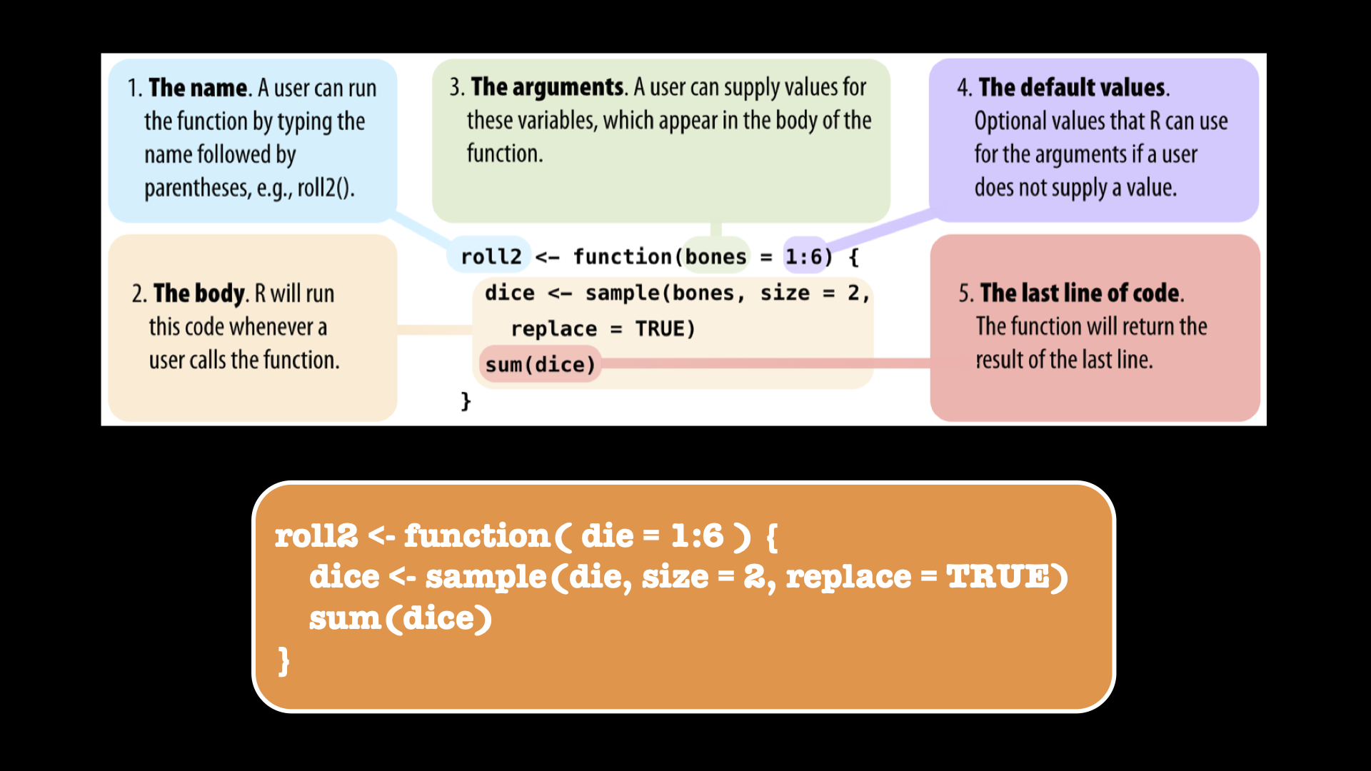
Figure 24.1: Create your own function.

roll2 <- function( die = 1:6 ) {
  dice <- sample(die, size = 2, replace = TRUE)
  sum(dice)
}

Let’s play:

roll2()
#> [1] 4

Roll the 2 dice as many times as the number of people in the room: who wins?

N = 12
replicate( N, roll2() )
#>  [1] 9 9 7 9 6 6 7 7 7 8 6 3

Roll the 2 dice to investigate the probability of each overall outcome:

library(ggplot2) # qplot function

rolls = replicate(1000, roll2())
ggplot2::qplot(rolls, binwidth = 1)
#> Warning: `qplot()` was deprecated in ggplot2 3.4.0.
#> This warning is displayed once every 8 hours.
#> Call `lifecycle::last_lifecycle_warnings()` to see where
#> this warning was generated.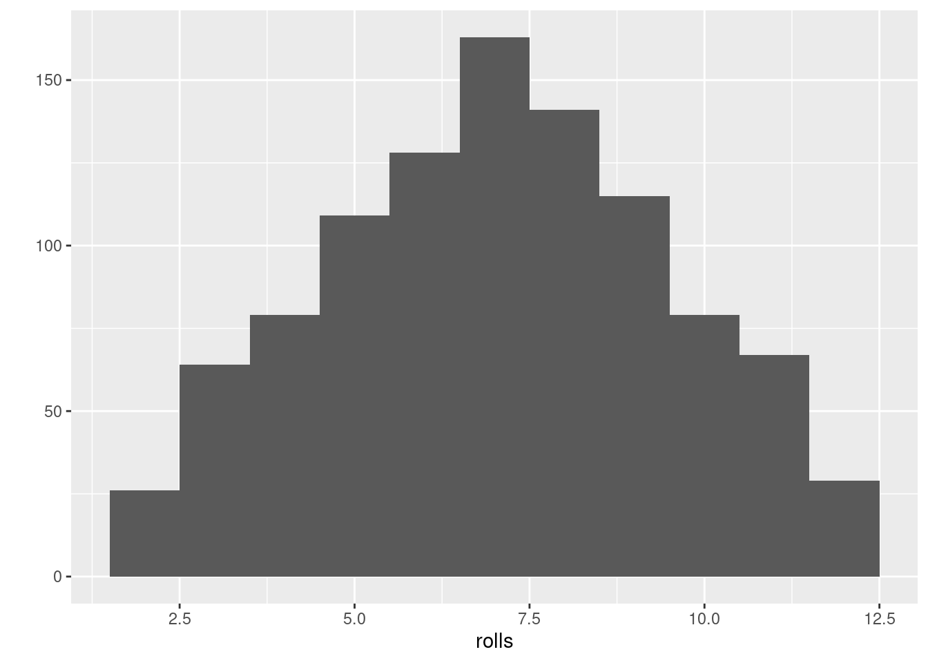

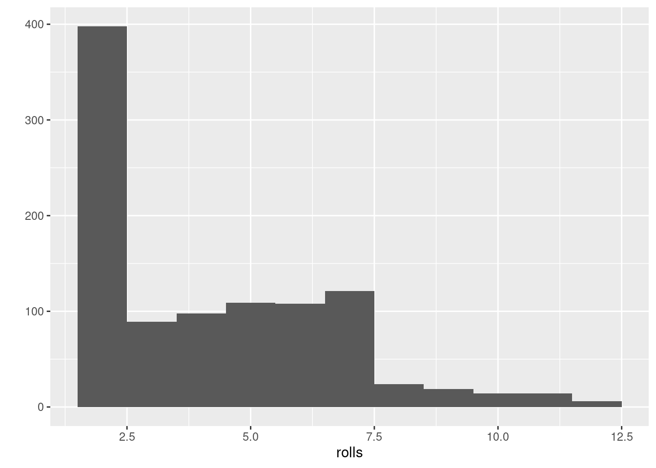
24.3.1.5 Let’s play using loaded dices

(Loaded dice = rigged die)

roll2_loaded <- function( die = 1:6 ) {
  dice <- sample( die, size = 2, replace = TRUE, 
                  prob=c(9/14,1/14,1/14,1/14,1/14,1/14) )
  sum(dice)
}

Roll the 2 dice to investigate the probabilities for loaded dice: Who wins?

rolls = replicate(1000, roll2_loaded())
qplot(rolls, binwidth = 1)

24.3.1.6 Assignment

Create a script and save it in the folder function_ex01 defined above including the following elaboration:

Create a new script
Save the script as name_surname_dice.R in the assigned folder
Write the following commands in the script:
- create a function to play with a die (a single die)
- roll the die 20 times
- store the results in a dedicated R object
- report the number of times the die returned each number from one to six.
- comment about the result
- is there at least one number which was more frequent?
- how many numbers and which were more frequent?

24.3.2 Create RMSE Error function

Objective: measure the goodness of a model.
Folder: ‘didattica/assignments/function_ex02/’

Create the following error function:

rmse <- function(M,P){
    # INPUTS
    #  M    : measurements
    #  P    : predictions
    
    # Checek that M & P have the same size:
    n1 <- length(M)
    n2 <- length(P)
    if(n1>n2 | n1<n2){
        print("Input vectors have different size!")
        return(NA)
    }
    
    n <- length(M)
    
    E = (M - P)
    S = E^2
    M = sum(S) / n
    R = sqrt(M)
    
    R # ---> return root mean square error
}

24.3.2.1 Assignment

Perform the following elaboration:

Create a new script and save it as name_surname_rmse.R in the folder function_ex02 defined above
Use the data provided in section height (H) and foot size (F) of students
Build a linear model between H (dep. var.) and F (indep. var.)
Interpolate the values of H given the F values provided
Measure the error of the model using the RMSE function created above

24.3.3 Create Pearson correlation function

Objective: measure the the level of linear dependence between two variables.
Folder: ‘didattica/assignments/function_ex03/’

Create the following error function:

myCorr = function(X,Y){
    nx = length(X)
    ny = length(Y)
    if (nx!=ny){
        stop('The length of inputs is different!')
    }else{
        n = nx
    }
    mu_x   = mean(X)
    mu_y   = mean(Y)
    COV_XY = sum( (X-mu_x)*(Y-mu_y) ) / n
    VAR_X  = sum( (X-mu_x)^2 ) / n
    VAR_Y  = sum( (Y-mu_y)^2 ) / n
    COV_XY / sqrt(VAR_X*VAR_Y) # --> return the correlation value
}

24.3.3.1 Assignment

Perform the following elaboration:

Create a new script
Import the soil temperature measurements provided in the file XY_Tmean.csv
Import the raster dem20m_campania.tif with elevation values for the whole Campania Region
Extract the elevation values from the raster at locations where the soil temperature values are available
Measure the level of linear dependence between the two variables soil temperature and elevation using the correlation function created above
save the script as name_surname_corr.R in the folder function_ex03 defined above

24.4 Collection and analysis of climatic data

Objective: Statistical manipulation of agrometeorological data.
Folder: ‘didattica/assignments/agrimeteo_ex01/’
Source: ISPRA > SCIA > Serie Temporali Giornaliere

24.4.1 Collection

You can download new data (temperature and precipitation) in CSV format from the link provided above.
Alternatively, use the temperature and precipitation data available in the two files:

Tmax.xlsx
Rainfall.xlsx

24.4.2 Compute the following statistics

After importing the data (downloaded from the portal or taken from the provided Excel files) into RStudio, perform the following elaborations:

reconstruct any missing data by computing the mean of the neighbourhood,
for the daily series of one year, compute the following statistics (for the monthly statistics, choose any month other than January):
- Maximum air temperature
  - Annual and monthly minimum value
  - Annual and monthly maximum value
  - Annual and monthly mean value
  - Compute the degree-days of a crop/insect of your choice
- Cumulative precipitation
  - Annual and monthly total rainfall
  - Annual and monthly number of rainy events
  - Rainiest weather perturbation (2 or more days) in the selected month

24.4.3 Reconstruction of missing temperature data at a station

Perform the following elaborations:

randomly select ( sample() ) 10 days of the year for one station
store in a separate R object (original <- ...) the temperature measurements of these 10 days
delete the 10 selected values by writing NO DATA VALUE,
build a linear regression model ( lm() ) between the selected station (dependent variable) and another one (independent variable) with a complete time series (or with no missing data on the 10 days that are missing in the dependent variable)
interpolate the missing values using the parameters of the linear regression model
compare the interpolated values with the original ones (object original) by computing the error
- compute the difference between the measured value and the predicted one
- compute the error (MSE or RMSE)

24.4.4 Assignment

Perform the following elaboration:

Create a new script
Fulfil the assignment provided in both Compute the following statistics and Reconstruction of missing temperature data at a station writing R commands in the script
Save the script as name_surname_soilT.R in the folder agrimeteo_ex01 defined above

24.5 Spatial interpolation

24.5.1 Few observations & manual interpolation

Objective: Spatial interpolation using basic R code and reasoning.
Folder: ‘didattica/assignments/spat_interp_ex01/’
Data: ‘didattica/docente_Langella/Data/xyCdDist.csv’ ; ‘didattica/docente_Langella/Data/xyCdDist_unknown.csv’

Please refer to the two CSV files listed under Data.

Use the cadmium concentration data provided in ‘xyCdDist.csv’ to perform spatial interpolations at the unknown location specified in ‘xyCdDist_unknown.csv’.

Develop an R script that implements the following spatial interpolation methods to predict the cadmium value at the unknown point:

Null model
Proximity polygon (Thiessen/Voronoi-based approach)
Nearest neighbors, using a maximum of 4 observations
Inverse Distance Weighting (IDW), using a maximum of 4 observations
Linear regression, using the variable dist (distance from the pollution source) as a predictor

Save and submit your script to the directory indicated under Folder above.

Tip: No additional libraries are required beyond base R. A bit of logical thinking will be enough to complete this exercise.

24.5.2 Cross-validation in single geospatial location

Objective: Spatial interpolation at one measured location.
Folder: ‘didattica/assignments/spat_interp_ex02/’
Data: ‘didattica/docente_Langella/Data/xyCdDist.csv’

Use the cadmium concentration data provided in ‘xyCdDist.csv’ to perform spatial interpolations at the geospatial location with row number 7.

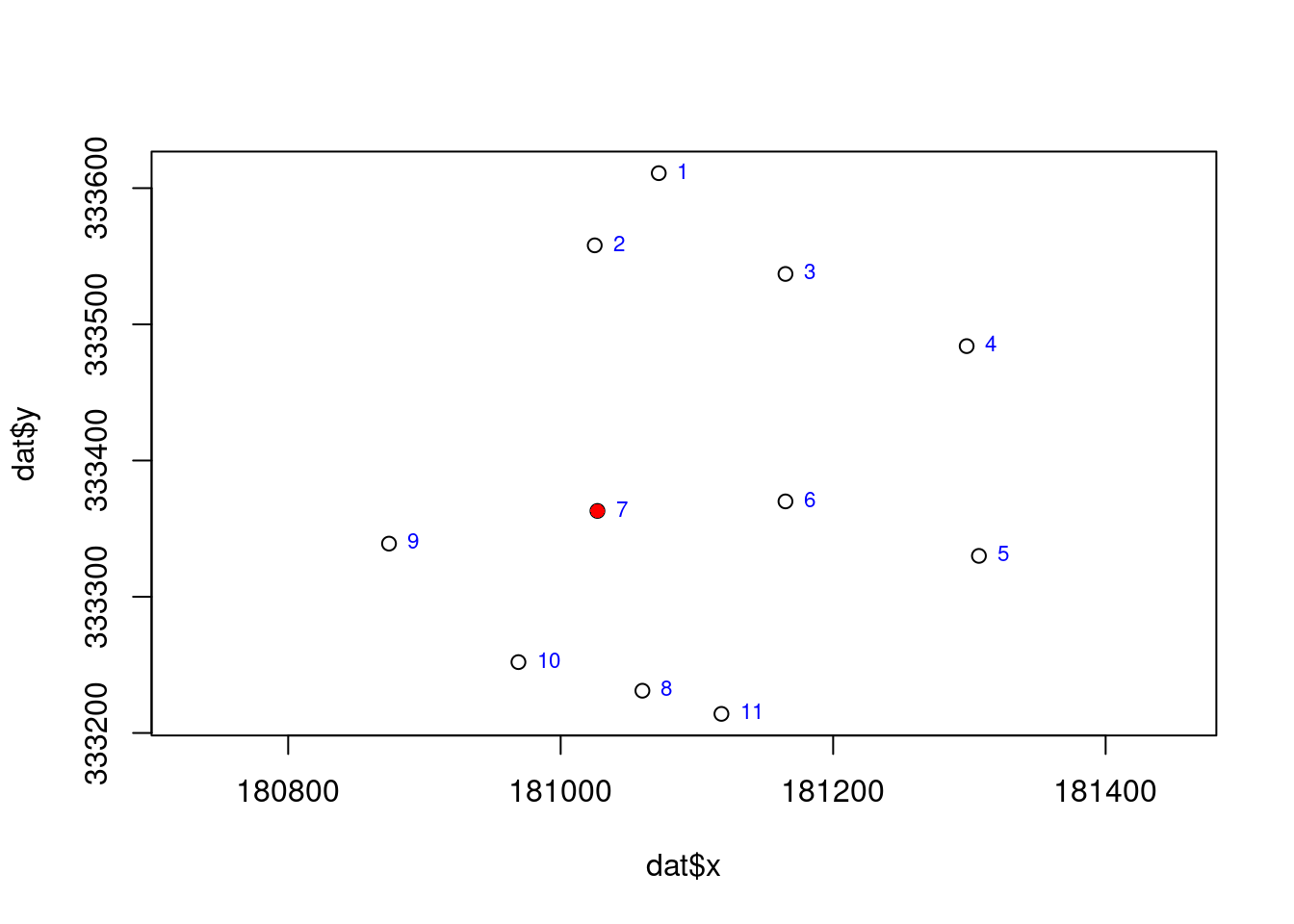
Develop an R script to implement the following spatial interpolation techniques for predicting cadmium concentration at the sampling point in row 7:

Null model
Proximity polygon (Thiessen/Voronoi-based approach)
Nearest neighbors, using a maximum of 4 observations
Inverse Distance Weighting (IDW), using a maximum of 4 observations
Linear regression, using the variable dist (distance from the pollution source) as a predictor

For each method, calculate the absolute error and decide about the most performing one.

Save and submit your script to the directory indicated under Folder above.

24.5.3 Cross-validation at all available geospatial locations

Objective: Spatial interpolation at all measured locations to enable cross validation.
Folder: ‘didattica/assignments/spat_interp_ex03/’
Data: ‘didattica/docente_Langella/Data/xyCdDist.csv’

Use the cadmium concentration data provided in ‘xyCdDist.csv’ to perform spatial interpolations at all geospatial locations. This exercise is identical to the previous one except that you have to extend what you did for measurement at row index 7 to all measurements.

Develop an R script to implement the following spatial interpolation techniques for predicting cadmium concentration at all sampling points:

Null model
Proximity polygon (Thiessen/Voronoi-based approach)
Nearest neighbors, using a maximum of 4 observations
Inverse Distance Weighting (IDW), using a maximum of 4 observations
Linear regression, using the variable dist (distance from the pollution source) as a predictor

For each method, calculate the RMSE and decide about the most performing one.

Save and submit your script to the directory indicated under Folder above.

24.6 Variography

24.6.1 Meuse assignment

Objective: Variography of meuse dataset and write commands and answers in a script.
Folder: ‘didattica/assignments/variography_ex01/’

Perform the following elaboration:

(load the required libraries)
Import the meuse built-in dataset
Analyse the content of object
- Which class?
- How many variables or attributes are available?
- How many records are available?
- Can you locate observations in spatial domain?
Transform into a simple feature
- Check in the help for the CRS
- Create a map using tmap to show the location of observations
- Do you find a relationship of contamination with the Meuse River?
- Describe this relationship…
Select a heavy metal different from Cadmium.
Create the cloud variogram and plot it
- print in console the object containing the information about the cloud variogram
- What does a single point in the chart represent? Explain in the script.
- Which point in the chart has the highest distance value? Write in the script the distance value.
- Which point in the chart has the highest variance value? Write the variance value in the script.
Create an experimental variogram and plot it
- print in console the object containing the information about the experimental variogram
- What does a single point in the chart represent? Explain in the script.
Perform a visual analysis of the experimental variogram in the chart and write the model variogram (using the vgm() function) which best fits the experimental one. This is a fitting made by eye.
- print in console the object containing the information about the model variogram fitted by eye
Plot the experimental variogram and the one fitted by eye.
Perform the automatic fitting (using the fit.variogram() function) of the experimental variogram
- print in console the object containing the information about the model variogram fitted automatically
Plot the experimental variogram and the one fitted automatically.
Compare the two model variograms fitted by eye and automatically: which one is working better and why?

Delivery

Create a new script
Fulfil the elaboration above
Save the script as name_surname_meuse.R (e.g. giuliano_langella_meuse.R) in the folder variography_ex01.

24.7 Regression tree

24.7.1 Assignment 1 — Introduction to Regression Trees

Objective:
Explore how to fit and interpret a regression tree using the BB.250 dataset.
The goal is to predict Soil Organic Carbon (SOC) based on available environmental covariates.

Folder: didattica/assignments/rtree_ex01/
Data: didattica/docente_Langella/Data/BB.250.csv

Load the BB.250 dataset and inspect its structure (e.g., str(), summary(), head()).
Build a regression tree model to predict SOC_target using the following predictors:
x_25833, y_25833, Altitude, Slope, NDVI, GNDVI, ERa, G_Total_Counts, B08, B02.
Plot the resulting tree and interpret its structure:
- Which variable is used at the root split?
- How many terminal nodes (leaves) are present?
- What is the predicted SOC value in each leaf?
Extract and display the variable importance from the model.
Visualize the predicted SOC values as a map using ggplot2, tmap, or another mapping package. Optionally, compare the predicted spatial pattern to the actual SOC values using a scatterplot or residual map.

Expected outcome:
A practical understanding of how regression trees partition space, how important covariates are selected, and how spatial predictions can be visualized and interpreted.

24.7.2 Assignment 2 — Model Evaluation and Comparison

Objective:
Evaluate the performance of a regression tree model by comparing it to simpler interpolation methods using a training/validation split and RMSE.

Folder: didattica/assignments/rtree_ex02/
Data: didattica/docente_Langella/Data/BB.250.csv

Split the BB.250 dataset into a training (80%) and validation (20%) subset using a random sampling strategy. Set a seed value to ensure reproducibility.
Fit a regression tree model on the training subset to predict SOC_target using the same predictors as in Assignment 1:
x_25833, y_25833, Altitude, Slope, NDVI, GNDVI, ERa, G_Total_Counts, B08, B02.
Predict SOC values at the validation locations using the fitted regression tree model, and compute the RMSE using a custom function (e.g., rmse_v3).
Compare the RMSE of the regression tree with that obtained from the following benchmark models:
- Global mean model: predict the mean SOC value from the training set for all validation points
- Nearest neighbour interpolation
- Inverse Distance Weighting (IDW)
Optionally, create maps of the residuals for each method to explore spatial patterns of under- or overestimation.

Expected outcome:
Ability to evaluate model accuracy using a validation subset, understand the limitations of global/statistical interpolators, and justify the use of machine learning approaches for spatial prediction.

23 Decision support