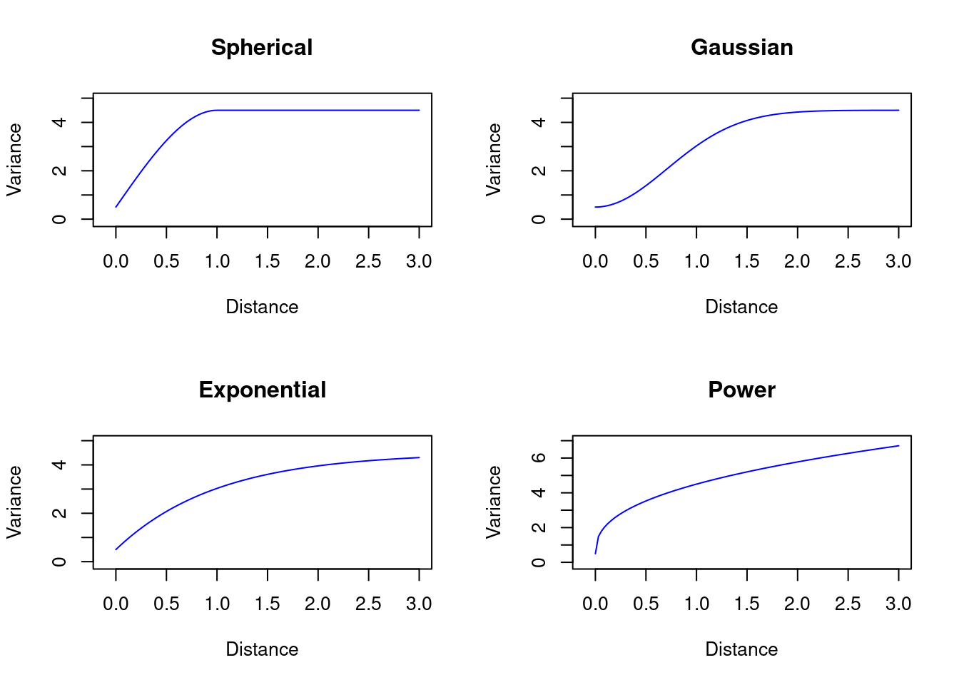
18 Variogram
Introduction to spatial statistical analysis by means of variography.
18.1 N O T E S
18.1.1 Notes about soil sampling:
- Extent/Scale of investigation;
- Geolocalization and density of sampling points;
- Sampling methods: soil profiles, (mini-)pits, boreholes, …;
- Objective of survey: observe localization and types of soils in the study area;
- Collection of soil samples, one (~1-2 kg) per soil horizon, for laboratory analysis (chemical, physical, …);
- Preparation data and exploratory statical analsys to enable the geostatistical analysis and modeling;
18.2 Build the Experimental Variogram
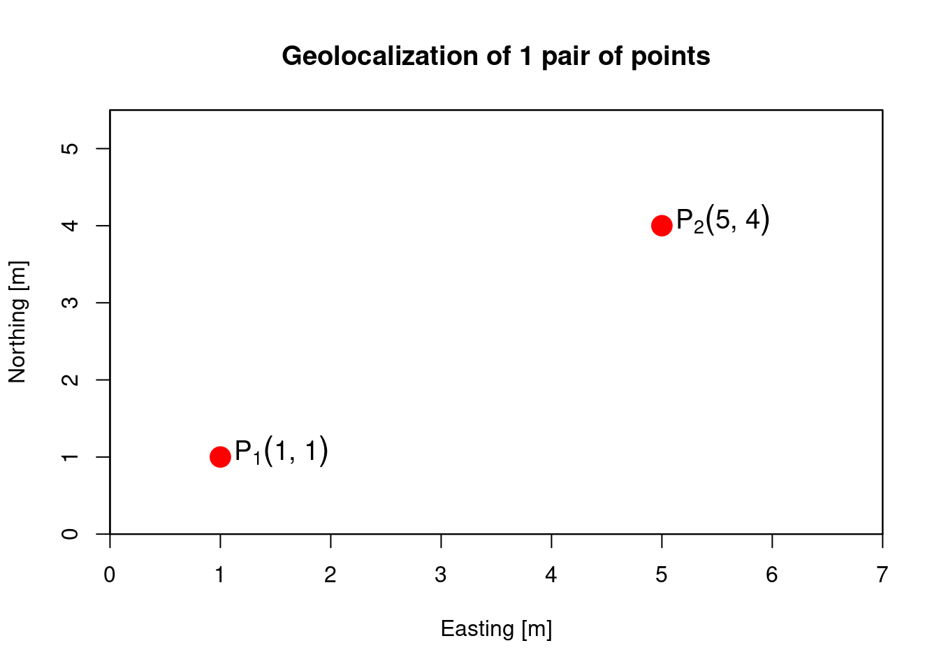
18.2.2 Graphical representation of sampling points
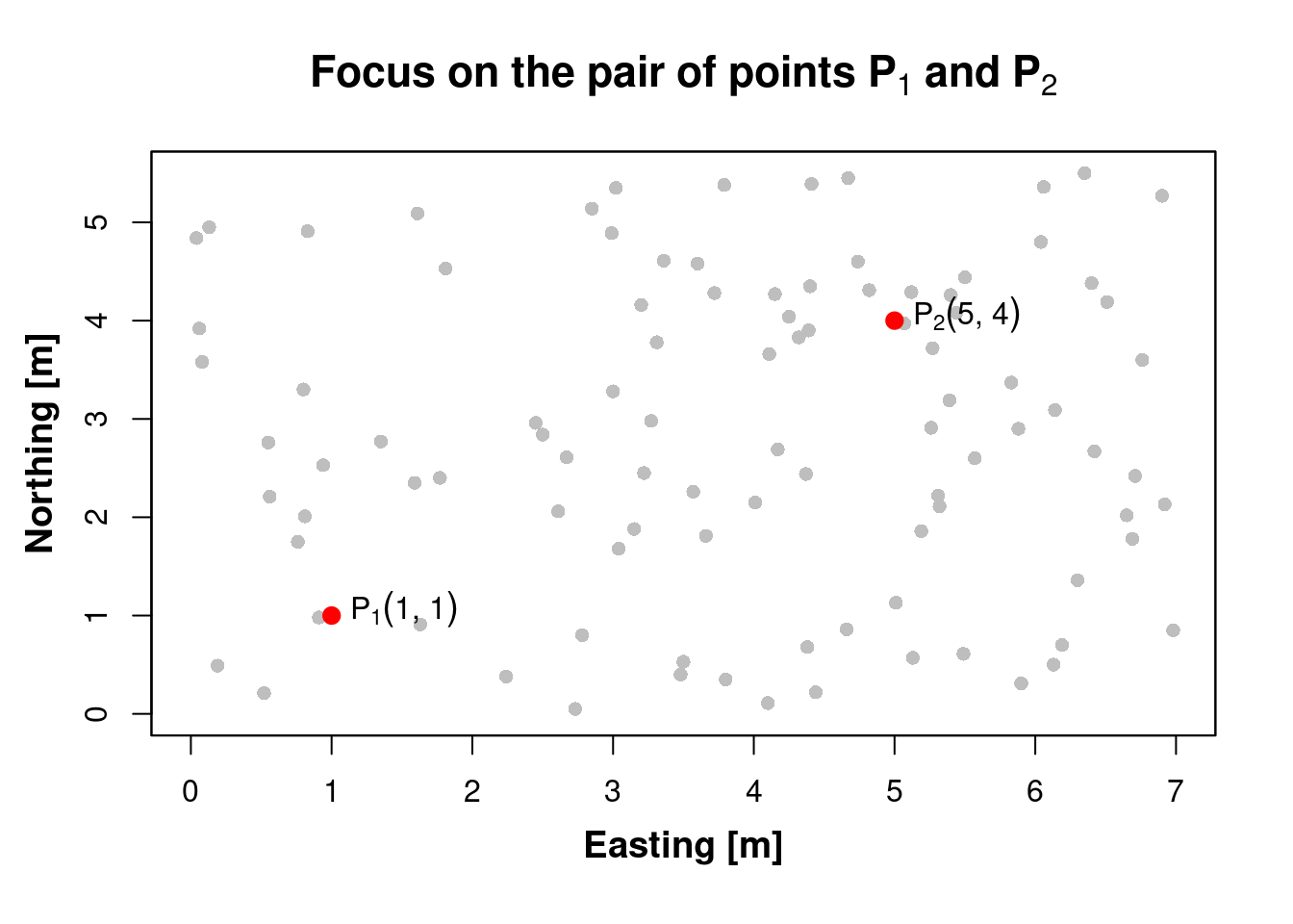
Create a pair of points, \(P_1(1,1)\) e \(P_2(5,4)\):
Create a vector of 100 points (that is an array of size \(100x1\)) with random and integer coordinates:
- X is in range [1,550]
- Y is in range [1,700]
- Division by 100 returns values in range 0 and 5.50(=X) or 7.00(=Y) with only 2 decimals.
# Generate random numbers with interval from 0 to 7.00
X <- sample(700, 100) / 100
# Generate random numbers with interval from 0 to 5.50
Y <- sample(550, 100) / 100
#>    Easting [m],   Northing [m]
#>           1.00,           1.00
#>           5.00,           4.00
#>           5.90,           0.31
#>           0.08,           3.58
#> 5.12, 4.29- having random values of Soil Organic Carbon \(\left[\frac{g}{kg}\right]\)
- as they were measured in topsoil (e.g. an \(A_p\) horizon or at fixed depth of 0-40 cm)
- (division by 1000 sets the values between 0.000 e 2.000 \(\frac{g}{kg}\))
Z <- sample(2000, 100, replace = TRUE) / 1000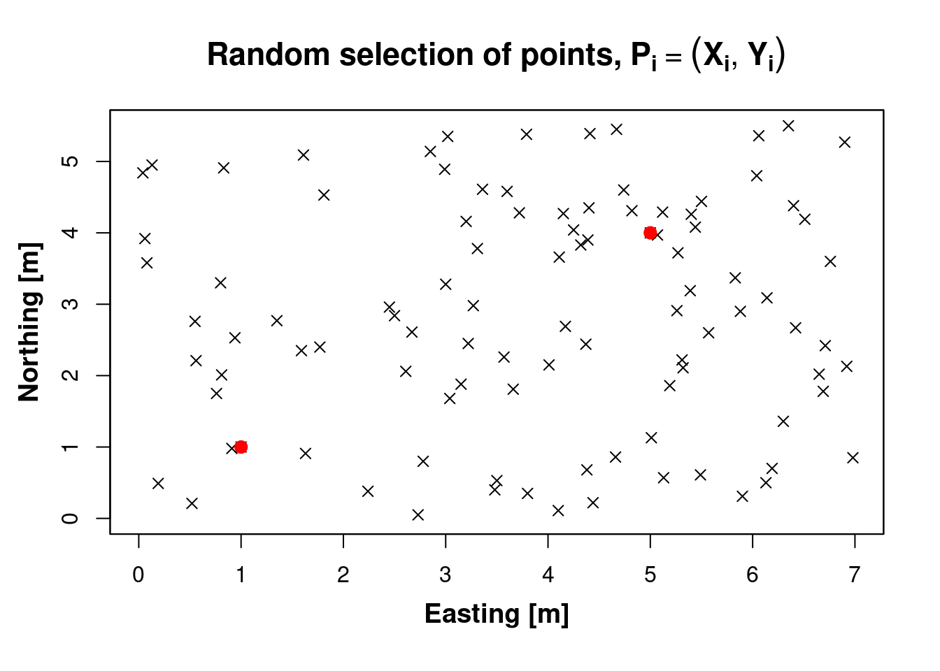
18.2.3 Focus on the first two points
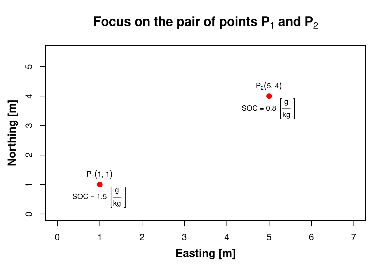
Locations \(P_1\) and \(P_2\) form a pair of geospatial points:
Each location has a distinct soil property value: for instance we focus on the amount of Soil Organic Carbon at horizon \(\color{blue}{\mathbf{A_{(p)}}}\):
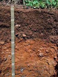
Figure 18.1: Soil Profile with horizons (e.g. at location \(P_1\)).
18.2.4 Objective: calculate the distance between two points \(\color{red}{\mathbf{P_1}}\) and \(\color{red}{\mathbf{P_2}}\)
- P O S I T I O N :: Geospatial distance between a pair of points (\(\color{red}{\mathbf{P_1}}\) and \(\color{red}{\mathbf{P_2}}\))
- Q U A N T I T Y :: “Distance” about the variable (soil property | S.O.C.) measured at the two locations \(\color{red}{\mathbf{P_1}}\) and \(\color{red}{\mathbf{P_2}}\)
- Calculate the euclidean distance between the two geospatial points \(\color{red}{\mathbf{P_1}}\) and \(\color{red}{\mathbf{P_2}}\)
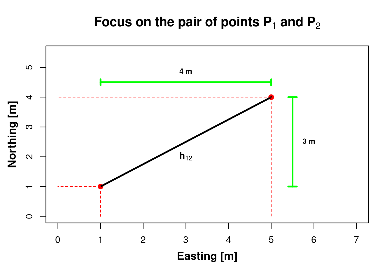
18.2.4.0.1 Pythagoras theorem:
\(h_{12} = \sqrt{(x_2-x_1)^2 + (y_2-y_1)^2} = \sqrt{4^2 + 3^2} = \sqrt{16 + 9} = \sqrt{25} = 5\) [m]
- Distance about S.O.C. [g/Kg] between the two geospatial points \(\color{red}{\mathbf{P_1}}\) and \(\color{red}{\mathbf{P_2}}\) [ V A R I A N C E ]
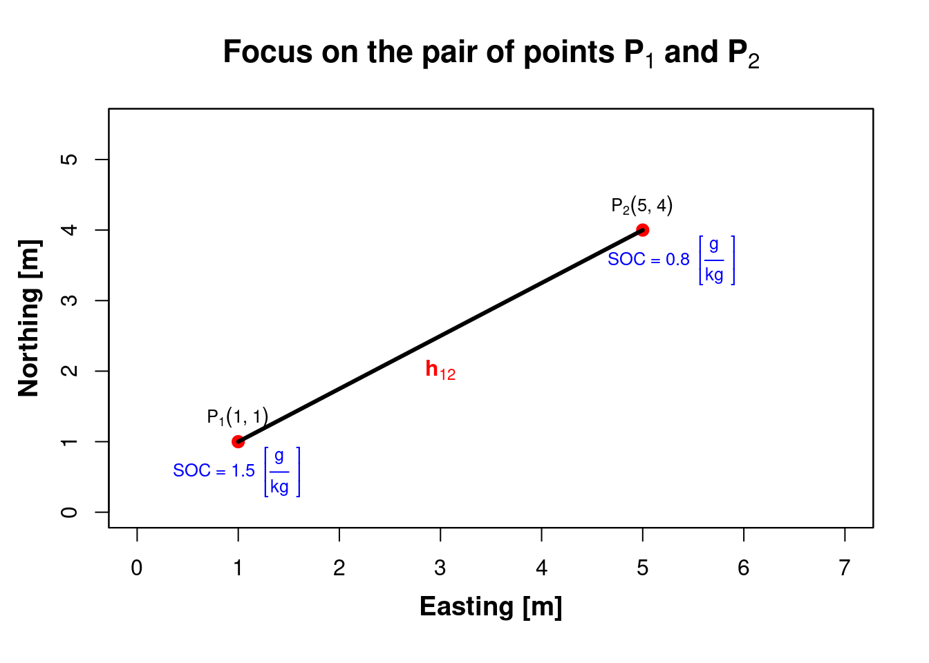
\(SOC_{P_1} = 1.5\,[g/Kg]\;\;\;\;–>\;z(P_{1}) = z(x_{i})\)
\(SOC_{P_2} = 0.8\,[g/Kg]\;\;\;\;–>\;z(P_{2}) = z(x_{i}+h)\)
Use \(\mathbf{z}\) to denote S.O.C. in soil horizons \(\color{blue}{\mathbf{A_p}}\),
but we can use \(\mathbf{z}\) to reference any other (soil) property.
\(\gamma (h_{12}) = \left(z\left(x_{1}+h_{12}\right)-z\left(x_{1}\right)\right)^{2} = (0.8 - 1.5)^2 = -0.7^2 = 0.49\)
z1 = 1.5 # g / kg
z2 = 0.8 # g / kg
gamma = (z2 - z1)^2
#> [1] "gamma = 0.49"
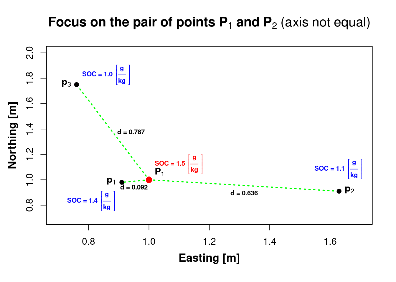
18.2.5 Extend the calculation to few points in the neibourhood of \(\color{red}{\mathbf{P_1}}\)
(fix point \(\color{red}{\mathbf{P_1}}\))
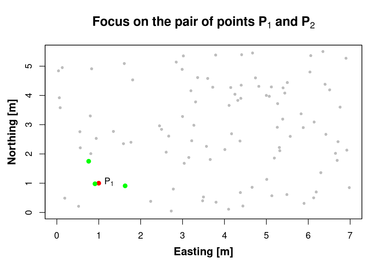
18.2.6 Calculate both geospatial distance and variance for the three pairs of measurements above
\(h_{1i} = \sqrt{(x_i-x_1)^2 + (y_i-y_1)^2}\)
\(\gamma (h_{1i}) = \left(z\left(x_{1}+h_{1i}\right)-z\left(x_{1}\right)\right)^{2}\)
distance = sqrt( (X[1] - xi)^2 + (Y[1] - yi)^2 )
variance = (Z[1] - zi)^2| distance | variance |
|---|---|
| 0.0921954 | 0.01 |
| 0.6363961 | 0.16 |
| 0.7874643 | 0.25 |
18.2.7 Extend the calculation to all sampling points…
- it means that we have to connect \(P_1\) to all other locations… (how many pairs we get if N location is 100?)
- …then we select \(P_2\) and connect it to all other locations…
- …then repeat till location \(P_{100}\).
- How many pairs can be built in total?
- How many pairs we get excluding the pairs made by the same point twice?
- How many duplicated pairs exist?
18.2.8 Cloud Variogram
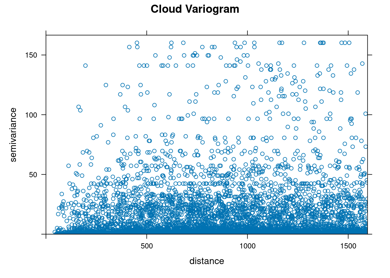
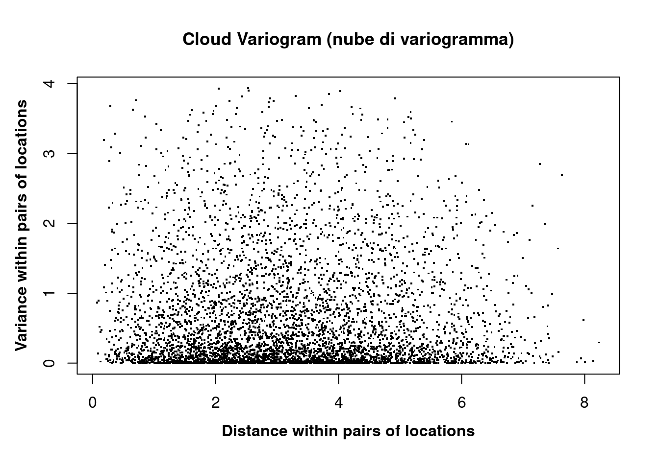
The scatterplot below is created using all pairs of locations that can be built using the whole dataset made by 100 locations.
 Questions
- Can you explain what does one single dot in the cloud variogram plot mean?
- Can you draw consistent considerations according to the cloud of points in the chart?
- Krige was studying an empirical solution observing this chart (see Wikipedia page about Danie Krige)
18.2.9 Experimental V A R I O G R A M
Let’s build the experimental variogram from the cloud variogram.
18.2.9.1 Lag and maximum distance
To build the experimental variogram we need to calculate two basic parameters following rules of thumb:- max distance (\(h_{max}\)) between 2 geospatial points separated by \(h\) → \(max\left(\frac{D}{2}\right)\)
- lag size → \(mean\left(min\left(D\right)\right)\)
Question: what is lag in geospatial context?
# hmax
hmax = max(D)/2      # rule of thumb #1

# lag
D2 = D
diag(D2) <- NA
rowMin = apply(D2, 1, FUN = min, na.rm=TRUE)
lag = mean(rowMin)   # rule of thumb #2

# N lag max
max_lags = floor(hmax/lag)
#> hmax = 4.119
#> lag = 0.332
#> Nlags = 1218.2.9.2 Separation of space using lags
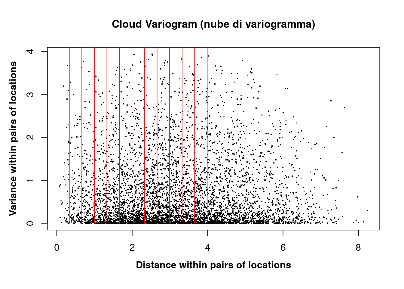
The cloud variogram is split into distinct regions according to growing ranges of distances between locations in the pairs.
In the plot below we have the cloud variogram (dots) and first 12 lags delimited by vertical red lines.
 NOTES
NOTES
- If we select the first lag (lag=1), we are considering all the pairs of locations separated by a vector \(h\) whose value is bounded between 0 and
0.3324018. - If we select the second lag (lag=2), we are considering all the pairs of locations separated by a vector \(h\) whose value is bounded between
0.3324018(\(1 \times lag\)) and0.6648036(\(2 \times lag\)). - …and so forth!
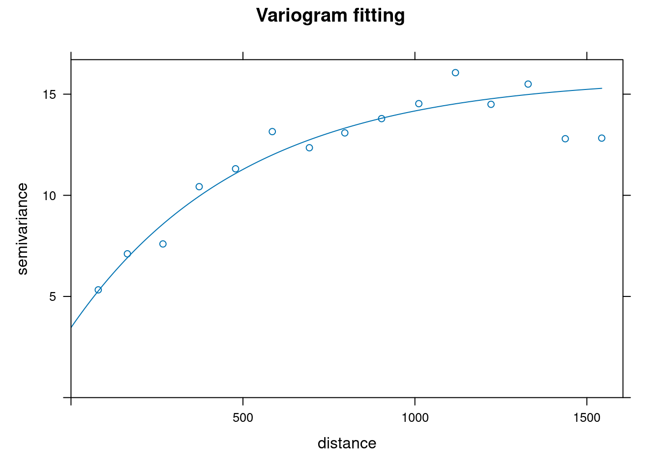
18.2.10 Experimental Variogram
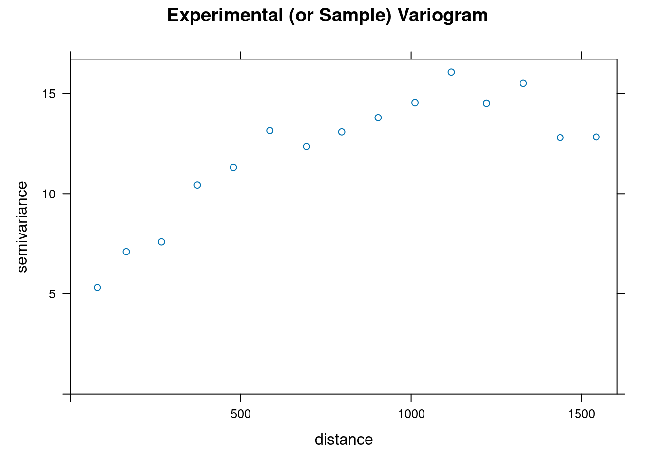
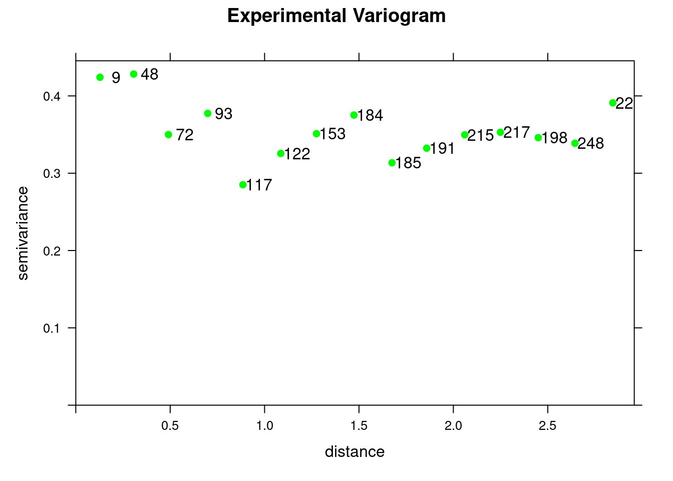
Following the work by Krige, we can aggregate the information of distance and variance available within each lag. Indeed, we can compute the mean distance and the mean variance for each lag. This way we simplifies the chart and we get the experimental variogram.
 NOTE:
NOTE:
- The experimental variogram above shows a pure nugget effect and the nugget correspondsto the variance \(C(0)\) (see next chapter on kriging).
QUESTIONS:
- What is the maximum distance on X axis? Is it lower than the maximum separation distance available in our dataset?
- Do you think that Tobler’s Law is verified with this plot? Why?
- Go back to the method used to generate the location and the SOC values of the sampling points: were they actually measured or synthetically created?
- Is there a possibility that the method used to generate both locations and SOC values affect the result in the chart? (analyse the pattern of varince with distance)
- Is there a trend in variance that can be explained using distance? Why?
18.2.11 Equation
Now we can derive the formula about the experimental variogram:
\({\displaystyle \gamma (h)=\sum _{i=1}^{n(h)}{\frac {(z(x_{i}+h)-z(x_{i}))^{2}}{n(h)}}}\)
NOTES:
- divide formula in blocks and focus on each one
- think of \(h\) as it were the lag and calculate the value of \(\gamma\) in your mind
18.2.11.1 Results of variogram calculations
| np | dist | gamma |
|---|---|---|
| 9 | 0.1280738 | 0.4240526 |
| 48 | 0.3066531 | 0.4282607 |
| 72 | 0.4908672 | 0.3499805 |
| 93 | 0.6987972 | 0.3773465 |
| 117 | 0.8853451 | 0.2851193 |
| 122 | 1.0855557 | 0.3255617 |
| 153 | 1.2753061 | 0.3511158 |
| 184 | 1.4733468 | 0.3752216 |
| 185 | 1.6748283 | 0.3135496 |
18.3 Main variogram characteristics
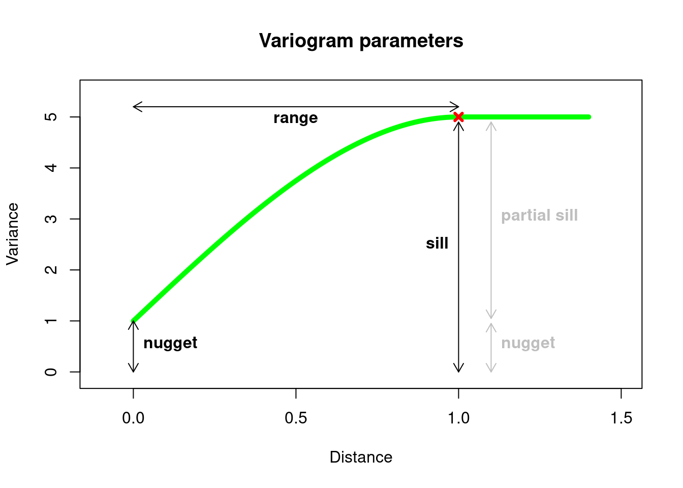
18.3.4 Variogram parameters
| Label | Parameter | Description |
|---|---|---|
| c0 | Nugget | the intesection of the variogram on the variance axes |
| a | Range | the projection of the variogram on the distance axes where the variance plateau begins |
| c | Sill | the projection of the variogram on the variance axes where the variance plateau begins |
| c - c0 | Partial Sill | the difference between the sill and the nugget |
18.3.6 Final reflections and closing insights
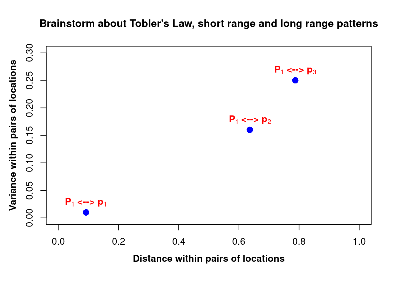
In the graph above, we are plotting the separation distance against the variance of three pairs of measurements.Some considerations come out:
- compare the overall pattern in the plot with the basic assumption in Tobler’s Law
- focus on the pattern of variance at short distance
- the less the distance (theoretically infinitesimal) the more the measurements are similar
- as the distance tends to infinitesimal, the measurements theoretically collapse to the same one
- the effect of sampling design on the statement above, i.e. the shortest distance available by sampling design sets a threshold in the data below which the pattern of spatial variability cannot be eplored
- focus on the pattern of variance at large distance
- the more the distance (theoretically infinite) the less the measurements are similar
- the basic principle above, which is implicit in Tobler’s Law, can be considered valid in case all disrupting events are cancelled out, such as a Volcano eruption or the footprint of humans (e.g. think to contamination)
