7 Geodata Visualization
Give a look to this interesting tutorial (vignette) written by Edzer Pebesma about Plotting Simple Features.
7.1 Basic plot function
The most important R function to plot data is called plot(). In most cases, it will manage particular classes by invoking the plot function available in the correspondent package.
7.1.1 Numeric Objects
A simple data frame can be plotted using base R:
x = rnorm(100)
y = rnorm(100)
plot(x, y,
     main = "Scatter Plot of Two Normally Distributed Random Variables",
     xlab = "X values",
     ylab = "Y values")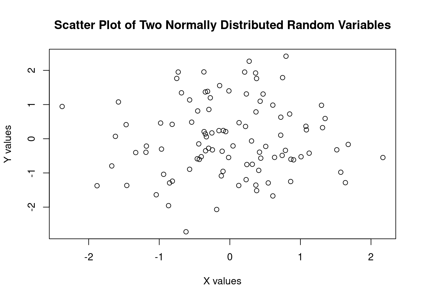
7.1.2 Data frame
Create the data frame reading a table from file:
library(readr)
soil_profiles <- read_table("datasets/Profile2.txt")
soil_profiles
#> # A tibble: 113 × 29
#>    SOIL_PROFILE  X_Coord  Y_Coord  clay d_tel slp_tel
#>    <chr>           <dbl>    <dbl> <dbl> <dbl>   <dbl>
#>  1 052P1        2485212. 4566397.  27.4   215   21.4
#>  2 052P2        2484993. 4567244.  30.1   306    8.84
#>  3 052P3        2484157. 4568470.  34.7   320    9.01
#>  4 052P4        2484006. 4566499.  26.1   207    9.72
#>  5 052P5        2485743. 4567682.  24.3   425   24.3
#>  6 052P6        2489992. 4563739.  25.3   125   33.3
#>  7 052P7        2484854. 4562926.  22.7    55    0
#>  8 052P8        2488026. 4564857.  14.5   156    5.66
#>  9 052P9        2479296. 4566807.  29.5   226    1.98
#> 10 052P10       2476558. 4560723.  23.6    59    4.76
#> # ℹ 103 more rows
#> # ℹ 23 more variables: aspct_tel <dbl>,
#> #   aspct_tel_linear <dbl>, t20b_T200_F15_gl <dbl>,
#> #   clc2k_tel <dbl>, il_acv_tel <dbl>, il_gchan_tel <dbl>,
#> #   il_gpeak_tel <dbl>, il_gpit_tel <dbl>,
#> #   il_gplai_tel <dbl>, il_gridg_tel <dbl>,
#> #   il_meanc_tel <dbl>, il_north_tel <dbl>, …
A data frame can be plotted using base R:
plot( soil_profiles$d_tel,
      soil_profiles$clay,
      main = "Scatter plot of clay vs elevation (Valle Telesina)",
      xlab = "Elevation [m]",
      ylab = "Clay [%]" )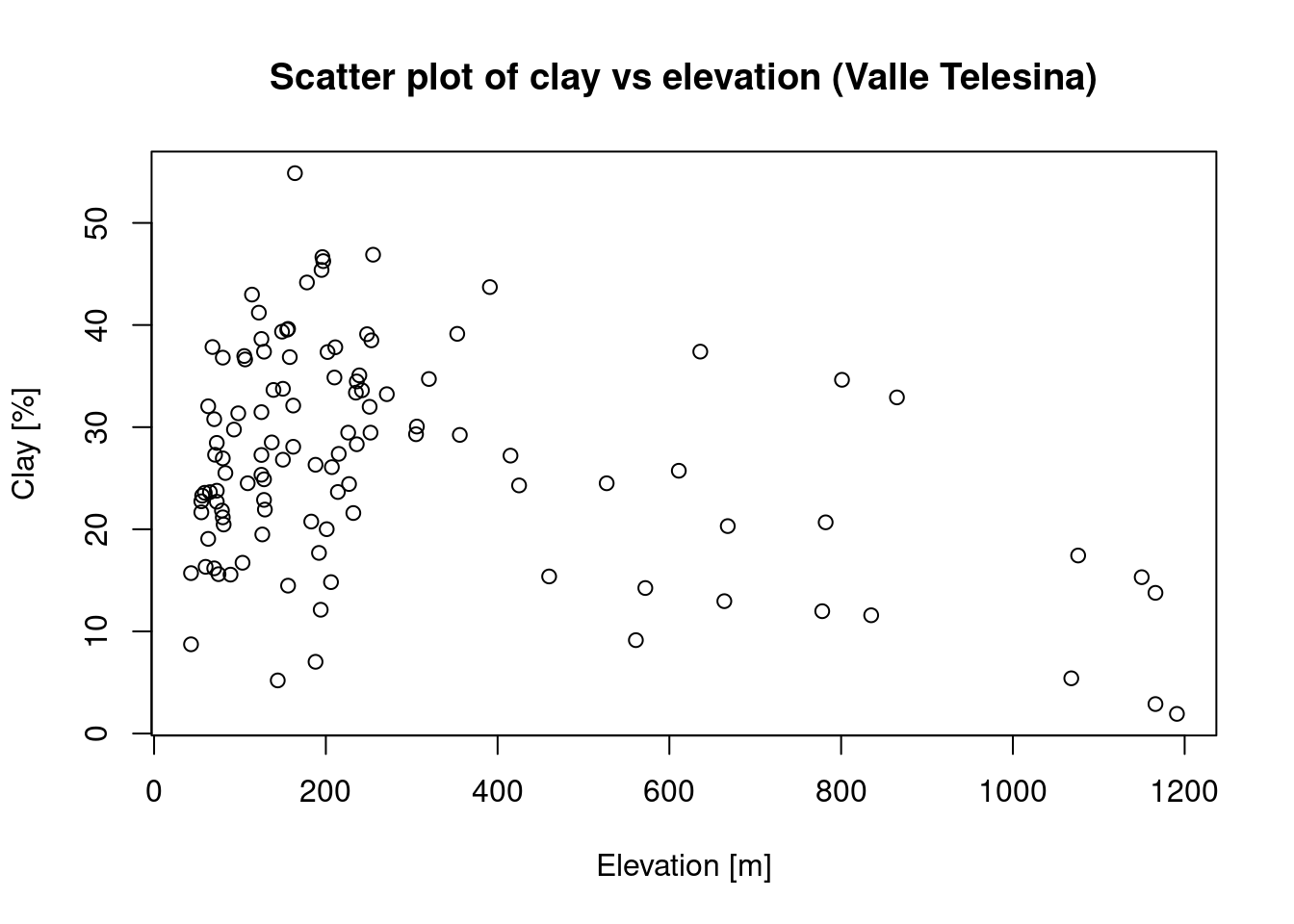
7.1.3 Simple Feature
Simple feature objects (sf) can be plotted directly with plot(). Different layers (geometry, attributes) are shown automatically in base plots:
library(sf)
Campania_region <- st_read("datasets/Ca.geojson")
#> Reading layer `Ca' from data source
#>   `/home/giuliano/lectures/datasets/Ca.geojson'
#>   using driver `GeoJSON'
#> Simple feature collection with 1 feature and 9 fields
#> Geometry type: MULTIPOLYGON
#> Dimension:     XY
#> Bounding box:  xmin: 13.76238 ymin: 39.99052 xmax: 15.80645 ymax: 41.50835
#> Geodetic CRS:  WGS 84
plot(Campania_region$geometry, main = "Campania region boundary")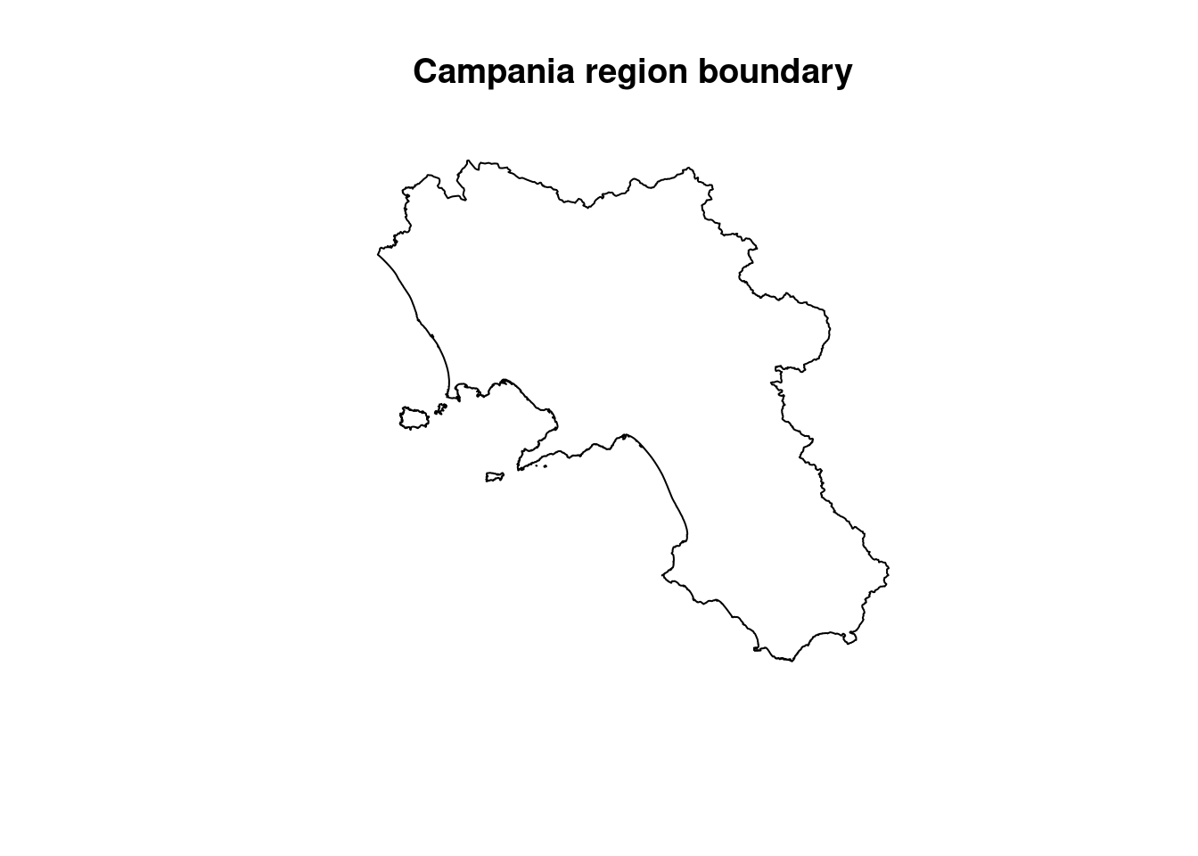
7.1.4 Raster
Raster layers from the terra package can also be visualized using plot():
library(terra)
r <- rast("datasets/ASTGTMV003_N02E042_dem.tif")
plot(r, main = "Elevation raster for Somalia (N02,E042)")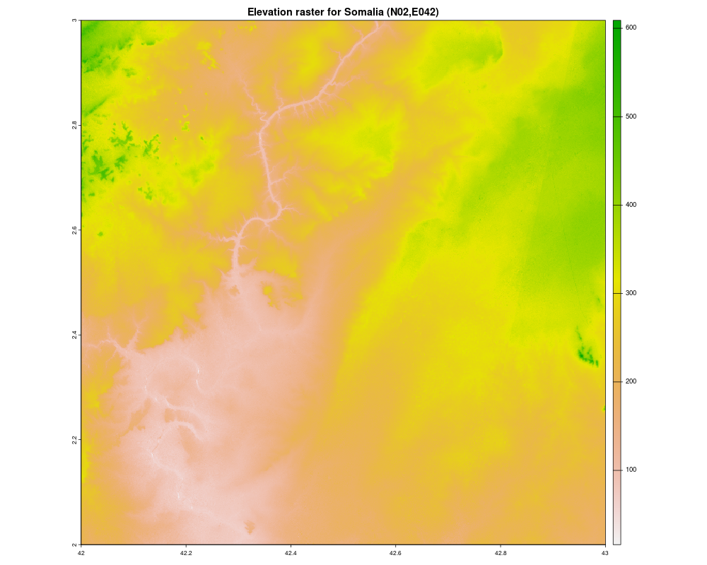
Figure 7.1: Elevation raster for Somalia (N02,E042)
We can also merge rasters to make a mosaic:
library(terra)

r1 <- rast("datasets/ASTGTMV003_N01E041_dem.tif")
r2 <- rast("datasets/ASTGTMV003_N01E042_dem.tif")
r3 <- rast("datasets/ASTGTMV003_N02E041_dem.tif")
r4 <- rast("datasets/ASTGTMV003_N02E042_dem.tif")

merged <- mosaic(r1, r2, r3, r4)

plot(merged, main = "Merged DEM tiles for Somalia")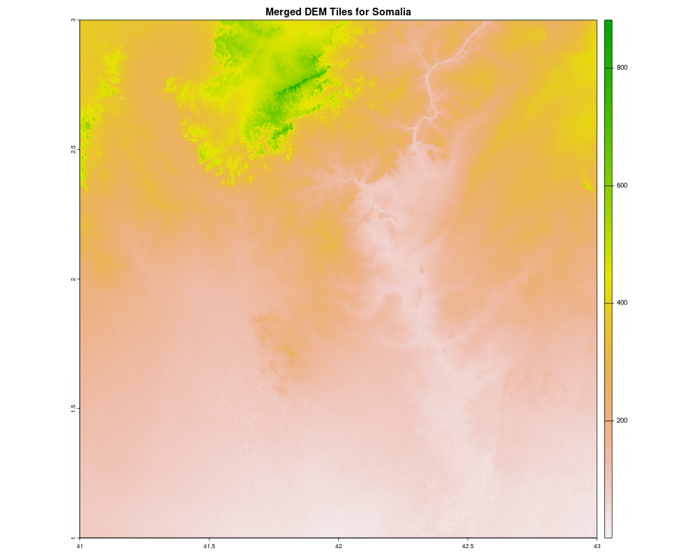
Figure 7.2: Merged DEM tiles for Somalia
7.2 Advanced ggplot2 library
The ggplot2 library provides more advanced and layered visualization options. With the help of geom_sf() or other geospatial-aware geoms, you can build elegant and customizable maps.
7.2.1 Example: Plotting sf data
library(ggplot2)
library(sf)

# Read the GeoJSON file
Campania_region <- st_read("datasets/Ca.geojson")
#> Reading layer `Ca' from data source
#>   `/home/giuliano/lectures/datasets/Ca.geojson'
#>   using driver `GeoJSON'
#> Simple feature collection with 1 feature and 9 fields
#> Geometry type: MULTIPOLYGON
#> Dimension:     XY
#> Bounding box:  xmin: 13.76238 ymin: 39.99052 xmax: 15.80645 ymax: 41.50835
#> Geodetic CRS:  WGS 84

# Plot using ggplot2
ggplot(data = Campania_region) +
  geom_sf(fill = "lightblue", color = "black") +
  theme_minimal() +
  labs(title = "Campania Region Boundary")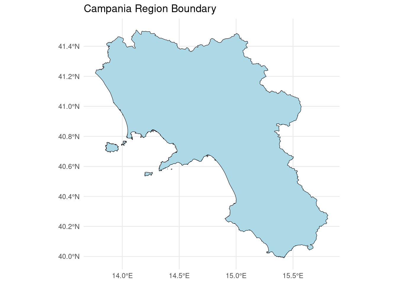
7.2.2 Example: Plotting a raster (as points)
For raster data, convert it to a data frame first:
library(terra)
library(ggplot2)

# Load the raster
r <- rast("datasets/ASTGTMV003_N02E042_dem.tif")

# Convert to data frame for ggplot2
r_df <- as.data.frame(r, xy = TRUE)

# Get the name of the raster layer (to use in aes)
names(r)
names(r_df)[3] <- "elevation"

# Plot using ggplot2
ggplot(r_df) +
  geom_raster(aes(x = x, y = y, fill = elevation)) +
  scale_fill_gradientn(colours = terrain.colors(10)) +
  theme_minimal() +
  labs(
    title = "Elevation Raster for Somalia (N02, E042) using ggplot.",
    x = "Longitude",
    y = "Latitude",
    fill = "Elevation (m)"
)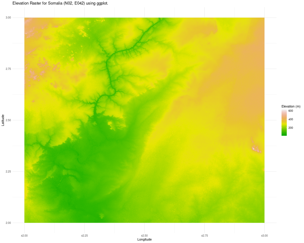
Figure 7.3: Elevation Raster for Somalia (N02, E042) using ggplot.
7.3 Advanced tmaps library
The tmap library allows the creation of either a static plot (mode=“plot”) or a dynamic plot (mode=“view”) with pan, zoom and data selection functionalities.
The mechanism is very simple since it work by adding layers one on top of the previous. Each layer is made by a combination of 2 functions:
-
tm_shape()is used to select the geodata (vector or raster) to show -
tm_*is used to set the specifics of the graphical representation of the selected geodata
Examples for the second function are grouped by the data model or geometry type:
- POINT:
tm_dots()ortm_bubbles() - POLYGON:
tm_polygons()ortm_borders - RASTER:
tm_raster()
Many arguments can be configured to customize the result of the map produced.
7.3.2 Create a map for POINT geometry
7.3.2.1 Import data
Create Air temperature measurements simple feature:
t_day <- read_csv("AirTemperature_day.csv")
t_day_sf <- st_as_sf(t_day,coords = c("lon","lat"), crs=4326)
Which variables are available?
names(t_day_sf)
#> [1] "Name"     "elev"     "mean"     "min"      "max"
#> [6] "N" "geometry"7.3.2.3 Bubbles
Let’s create a map using the tmap library:
tmap::tmap_mode("view")
tm_shape(t_day_sf) +
  tm_bubbles(size="max",col="elev")
7.3.3 Create a map for (MULTI)POLYGON geometry
7.3.3.1 Borders
# Read the GeoJSON file
Campania_region <- st_read("datasets/Ca.geojson",quiet=TRUE)

tmap::tmap_mode("view")
tm_shape(Campania_region) +
tm_borders(col="red",lwd=3)7.3.4 Raster
7.3.4.1 Static raster plot:
library(terra)
library(tmap)

dem <- rast("datasets/ASTGTMV003_N02E042_dem.tif")

tmap_mode("plot")
tm_basemap("OpenTopoMap") +
  tm_shape(dem) +
  tm_raster(palette = "-viridis")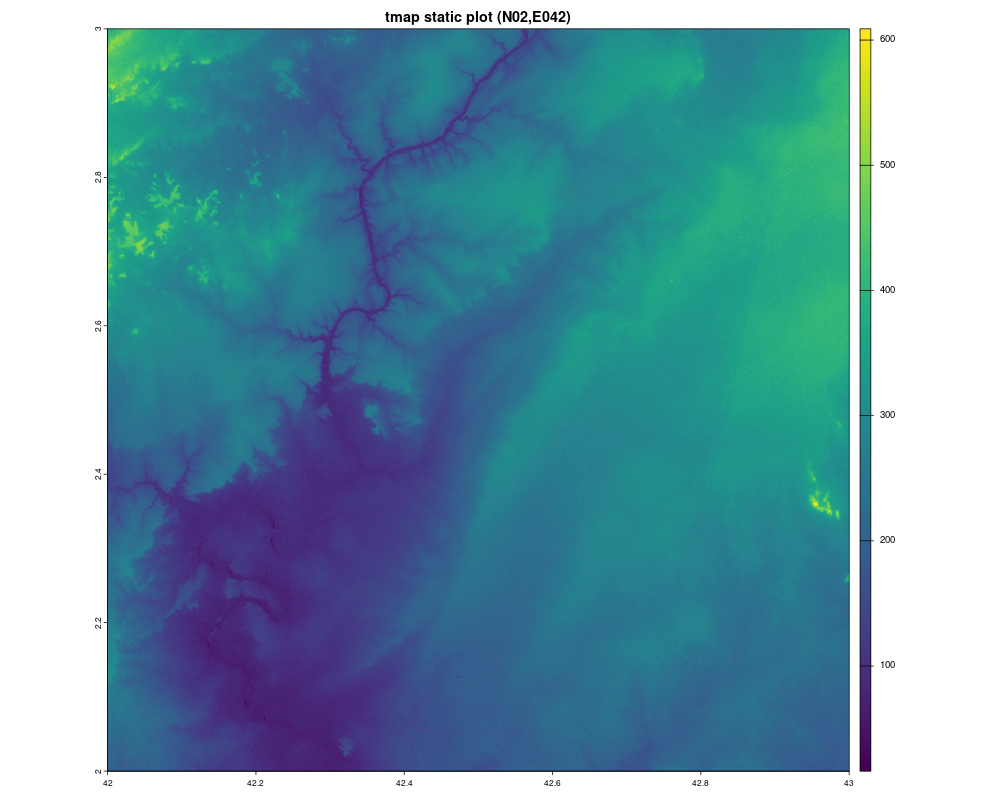
Figure 7.4: Elevation raster for Somalia (N02,E042)
7.3.4.2 Interactive raster view:
library(tmap)
library(terra)

dem <- rast("datasets/ASTGTMV003_N02E042_dem_small.tif")

tmap_mode("view")
tm_basemap("OpenTopoMap") +
  tm_shape(dem) +
  tm_raster(palette=terrain.colors(20))
7.3.5 Basemaps available
When working with tmap in interactive mode (using tmap_mode(“view”)), you can add online basemaps as background layers. These basemaps come from the Leaflet Providers collection and can be explored here:
https://leaflet-extras.github.io/leaflet-providers/preview/
To use a basemap in tmap, you simply specify its provider name inside the tm_basemap() function. Below is a short list of recommended basemaps for this course:
OpenTopoMap
Clean topographic background suitable for elevation and terrain analysis.
Example: tm_basemap("OpenTopoMap")
Esri.WorldPhysical
Soft physical map showing landforms and terrain morphology.
Example: tm_basemap("Esri.WorldPhysical")
Esri.WorldImagery (Satellite)
High-resolution satellite basemap, ideal for visual comparison with ground features.
Example: tm_basemap("Esri.WorldImagery")
OpenStreetMap
Standard street-level map with clear labels and features.
Example: tm_basemap("OpenStreetMap")
These basemaps can be combined with your spatial layers (both raster and vector data) to create rich and informative visualizations in interactive mode.
7.4 Geobounds library
The geobounds package provides an R-friendly interface to access and work with the geoBoundaries dataset (an open-license global database of administrative boundary polygons).
7.4.1 Italy
Get the boundary for Italy:
library(geobounds)
italia = gb_get_adm0("ITA")
italia
Simple feature collection with 1 feature and 5 fields
Geometry type: MULTIPOLYGON
Dimension:     XY
Bounding box:  xmin: 6.626621 ymin: 35.49285 xmax: 18.52038 ymax: 47.09178
Geodetic CRS:  WGS 84
# A tibble: 1 × 6
  shapeName  shapeISO shapeID           shapeGroup shapeType
* <chr>      <chr>    <chr>             <chr>      <chr>
1 Nord-Ovest <NA>     42024856B8524037… ITA        ADM0
# ℹ 1 more variable: geometry <MULTIPOLYGON [°]>
Set line width using the lwd argument:
tmap_mode("plot")
tm_basemap("OpenStreetMap") +
tm_shape(italia) +
tm_borders(col="brown",lwd=2) 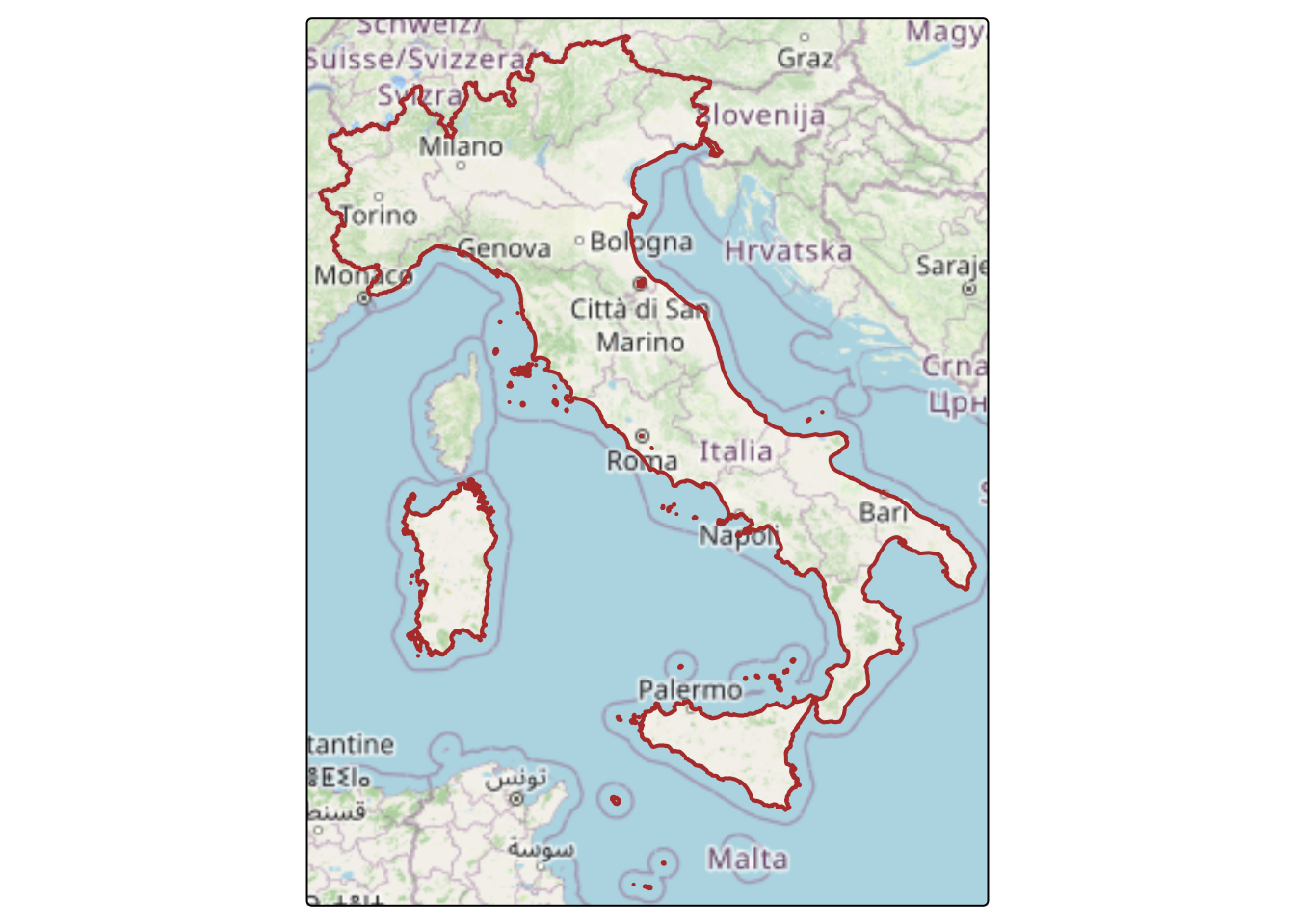 Get regions in Italy:
regioni <- gb_get_adm2("ITA")Plot regions:
tmap_mode("plot")
tm_shape(regioni) + tm_polygons(fill = "shapeName") +
  tm_shape(italia) + tm_borders(col="black",lwd=2)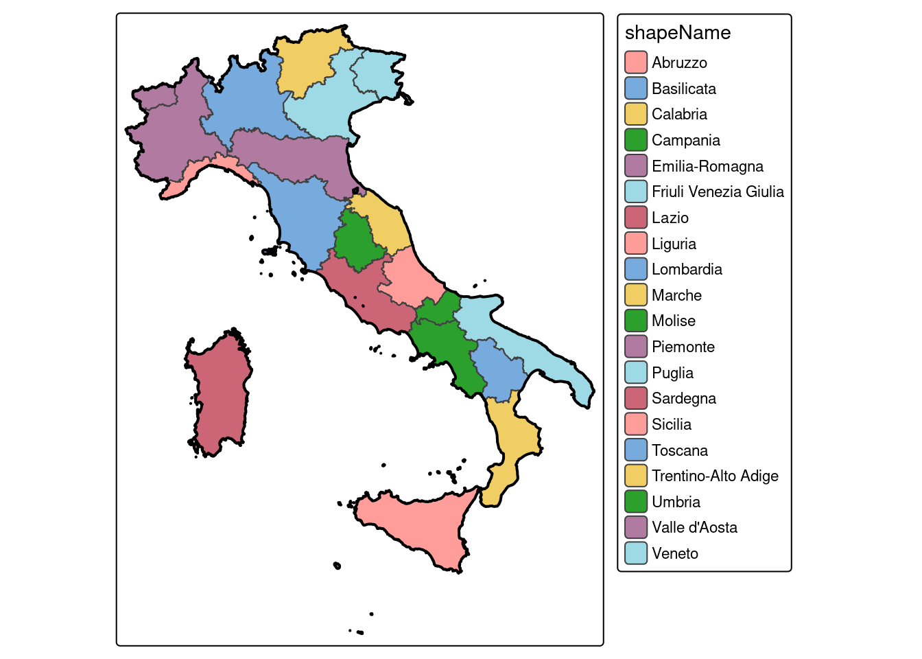
7.5 Geodata library
geodata is an R package for downloading geographic data. This package facilitates access to climate, elevation, soil, crop, species occurrence, and administrative boundary data, and is a successor of the getData() function from the raster package.
The reference documentation is available for full reference to functions.
Let’s carry out some examples about elevation, cropland and soils.
7.5.1 Elevation
it_s <- elevation_3s(14.8, 40.3, path=tempdir())
#> Cached as: /tmp/RtmpPoN7Xv/elevation/srtm_39_04.ZIP
it_s
#> class       : SpatRaster
#> dimensions  : 6000, 6000, 1  (nrow, ncol, nlyr)
#> resolution  : 0.0008333333, 0.0008333333  (x, y)
#> extent      : 10, 15, 40, 45  (xmin, xmax, ymin, ymax)
#> coord. ref. : +proj=longlat +datum=WGS84 +no_defs
#> source      : srtm_39_04.tif
#> name        : srtm_39_04
plot(it_s)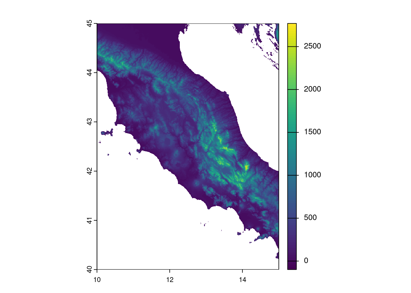
7.5.2 Cropland
cropland( source="worldcover",
          year=2019,
          path="/home/giuliano/datasets/WorldCover_cropland_30s.tif"
        )
cl19 <- rast("/home/giuliano/datasets/WorldCover_cropland_30s.tif")
cl19
#> class       : SpatRaster
#> dimensions  : 17280, 43200, 1  (nrow, ncol, nlyr)
#> resolution  : 0.008333333, 0.008333333  (x, y)
#> extent      : -180, 180, -60, 84  (xmin, xmax, ymin, ymax)
#> coord. ref. : lon/lat WGS 84 (EPSG:4326)
#> source      : WorldCover_cropland_30s.tif
#> name        : cropland
#> min value   :        0
#> max value   :        1
plot(cl19)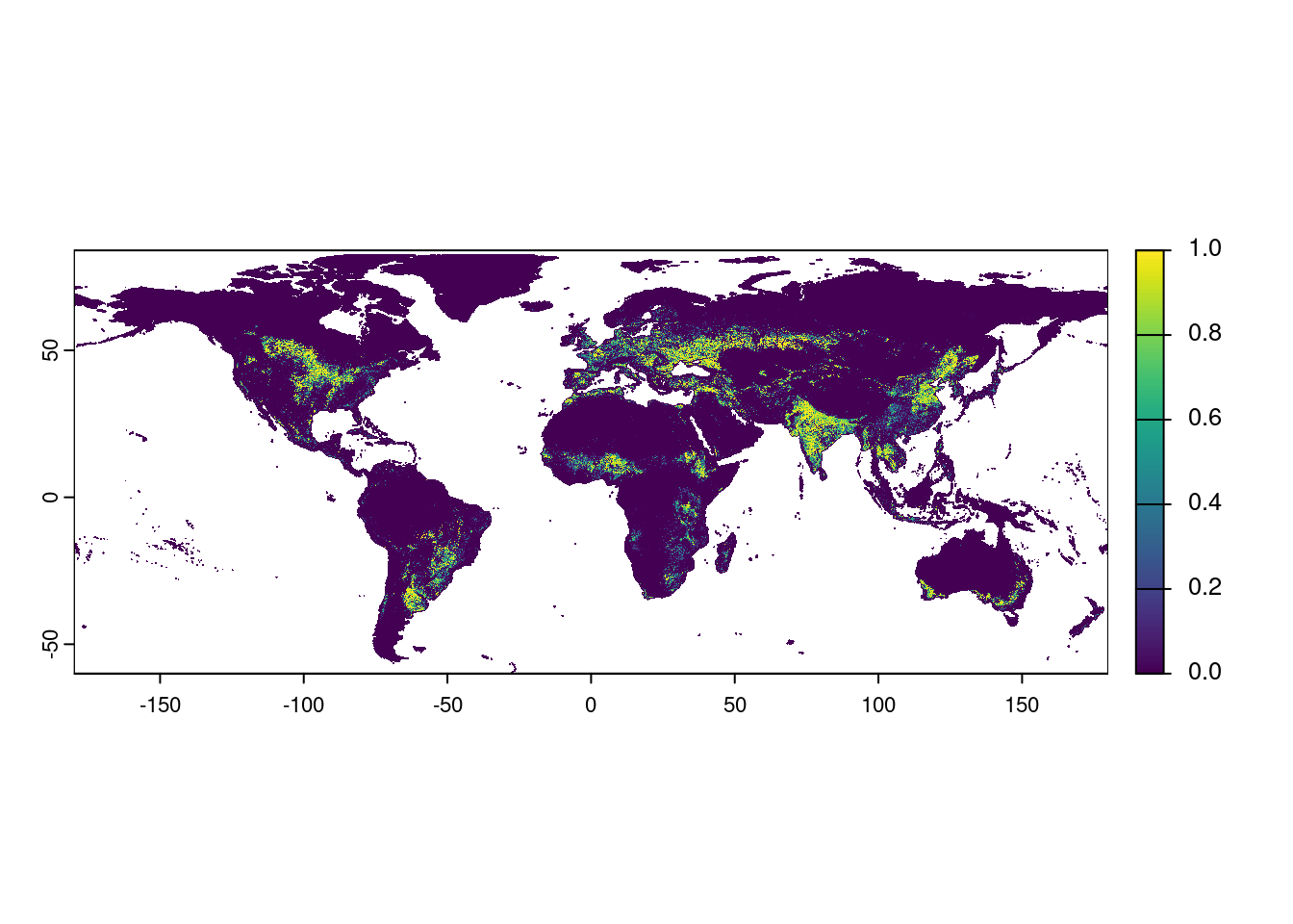
Get Italy boundaries:
italy = gb_get_adm0("ITA")Check that both geodata - Italy boundaries (vector data) and World cropland (raster data) - have the same CRS:
Select (GIS crop operation) Italy from cropland data:
cl19_it <- terra::crop(cl19,italy)
cl19_it
#> class       : SpatRaster
#> dimensions  : 1392, 1427, 1  (nrow, ncol, nlyr)
#> resolution  : 0.008333333, 0.008333333  (x, y)
#> extent      : 6.625, 18.51667, 35.49167, 47.09167  (xmin, xmax, ymin, ymax)
#> coord. ref. : lon/lat WGS 84 (EPSG:4326)
#> source(s)   : memory
#> varname     : WorldCover_cropland_30s
#> name        : cropland
#> min value   :        0
#> max value : 17.5.3 Soils
soil_world( var="bdod",
            depth=15,
            stat="mean",
            path="/home/giuliano/datasets/bdod_5-15cm_mean_30s.tif"
          )
Import:
bd15mean <- rast("/home/giuliano/datasets/bdod_5-15cm_mean_30s.tif")
bd15mean
Crop raster data to Italy boundaries:
## bd15mean_it <- crop(bd15mean,italy)
bd15mean_it
#> class       : SpatRaster
#> dimensions  : 1392, 1427, 1  (nrow, ncol, nlyr)
#> resolution  : 0.008333333, 0.008333333  (x, y)
#> extent      : 6.625, 18.51667, 35.49167, 47.09167  (xmin, xmax, ymin, ymax)
#> coord. ref. : lon/lat WGS 84 (EPSG:4326)
#> source      : bd15mean_it.tif
#> name        : bdod_5-15cm
#> min value   :         0.7
#> max value   :         1.7
Plot soil bulk density:
plot(bd15mean_it)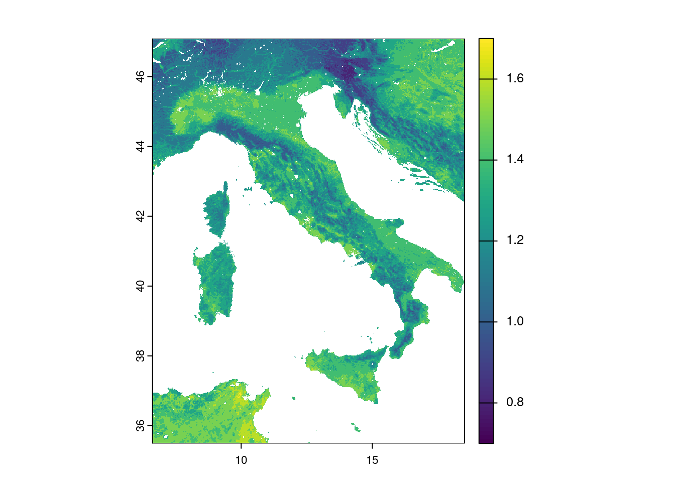
7.6 Animating views
library(plotly)
library(htmlwidgets)
library(gapminder)

p <- plot_ly(x = rnorm(100))

data(gapminder, package = "gapminder")
gg <- ggplot(gapminder, aes(gdpPercap, lifeExp, color = continent)) +
  geom_point(aes(size = pop, frame = year, ids = country)) +
  scale_x_log10()
ggplotly(gg)
7.6.1 Note
Note that you learnt how to create interactive maps using the "view" mode.
In the book GEOG3915 GeoComputation and Spatial Analysis practicals by Lex Comber more examples can be found.