16 Inverse Distance Weighting

16.1 Basic form of the equation

\({\large\hat{z}({\mathbf u}) = \displaystyle\sum_{\alpha=1}^{n({\mathbf u})} \lambda_{\alpha}({\mathbf u}) z({\mathbf u}_{\alpha})}\)

\({\large\lambda_{\alpha}({\mathbf u}) = \frac{w_{\alpha}}{\sum_{\alpha=1}^{n({\mathbf u})}w_{\alpha}}}\)

\({\LARGE w_{\alpha} = \frac{1}{d^p\left(x_{\alpha},x_u\right)} }\)

Weights must sum up to one:

\({\large \sum_{\alpha=1}^{n({\mathbf u})} \lambda_{\alpha}({\mathbf u}) = 1}\)

16.1.1 An example

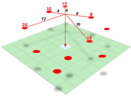
ToDo: add a plot with three points used in the example below

16.1.1.1 About weigths \(w_i\ldots\)

w <- c(8, 6, 3)

w[1]/sum(w)
#> [1] 0.4705882

w[2]/sum(w)
#> [1] 0.3529412

w[3]/sum(w)
#> [1] 0.1764706

The amount of all weights together must be equal to 1, in order to be congruent with measurements.

(w[1] + w[2] + w[3])/sum(w)
#> [1] 1

16.1.1.2 About measurements \(z_i \ldots\)

z <- c(40, 30, 20)

16.1.1.3 What happens if we have only one point contributing to the interpolation of the unknow value \(z_u\) at point location \(x_u\)?

w <- c(8, 0, 0)

zu <- sum(z * w/sum(w))
zu
#> [1] 40

16.1.1.4 What happens if we have only two points contributing to the interpolation of the unknow value \(z_u\) at point location \(x_u\)?

w <- c(8, 6, 0)

zu <- sum(z * w/sum(w))
round(zu, 1)
#> [1] 35.7

16.1.1.5 What happens if we invert the weights given to measured points?

w <- c(6, 8, 0)

zu <- sum(z * w/sum(w))
round(zu, 1)
#> [1] 34.3

16.1.1.6 Consider all the points contributing to the interpolation of the unknow value \(z_u\) at point location \(x_u\)?

w <- c(8, 6, 3)

zu <- sum(z * w/sum(w))
round(zu, 1)
#> [1] 32.9

16.1.1.7 What happens if we invert the weights given to all measured points?

w <- c(3, 6, 8)

zu <- sum(z * w/sum(w))
round(zu, 1)
#> [1] 27.1

16.2 Application of the method on a real problem

16.2.1 Import XT_Tmean.csv

library(readr)
tmean <- read.csv("XY_Tmean.csv")

class(tmean)
#> [1] "data.frame"

16.2.1.1 Convert the dataframe into Simple Feature

Use the sf package to convert a data frame into a simple feature:

library(sf)
#> Linking to GEOS 3.10.2, GDAL 3.4.1, PROJ 8.2.1; sf_use_s2()
#> is TRUE
tmean_sf <- st_as_sf(tmean, coords = c("Xcoord", "Ycoord"), crs=32633)

16.2.1.2 Map

Visualize data using the tmap library and the interactive mode (tmap_mode("view")):

# load library:
library(tmap)

# configure the tmap lib to work using interactive maps:
tmap_mode("view")
#> ℹ tmap mode set to "view".

# create the map using each layer on top of the previous one:
tm_shape(tmean_sf) + 
  tm_dots()

16.2.1.3 Summary

summary(tmean_sf)
#>      Tmean                  geometry  
#>  Min.   : 0.3347   POINT        :493  
#>  1st Qu.: 1.4522   epsg:32633   :  0  
#>  Median : 3.2497   +proj=utm ...:  0  
#>  Mean   : 3.5548                      
#>  3rd Qu.: 5.0767                      
#>  Max.   :12.6371

This is the CRS of the simple feature tmean_sf:

st_crs(tmean_sf)
#> Coordinate Reference System:
#>   User input: EPSG:32633 
#>   wkt:
#> PROJCRS["WGS 84 / UTM zone 33N",
#>     BASEGEOGCRS["WGS 84",
#>         ENSEMBLE["World Geodetic System 1984 ensemble",
#>             MEMBER["World Geodetic System 1984 (Transit)"],
#>             MEMBER["World Geodetic System 1984 (G730)"],
#>             MEMBER["World Geodetic System 1984 (G873)"],
#>             MEMBER["World Geodetic System 1984 (G1150)"],
#>             MEMBER["World Geodetic System 1984 (G1674)"],
#>             MEMBER["World Geodetic System 1984 (G1762)"],
#>             MEMBER["World Geodetic System 1984 (G2139)"],
#>             ELLIPSOID["WGS 84",6378137,298.257223563,
#>                 LENGTHUNIT["metre",1]],
#>             ENSEMBLEACCURACY[2.0]],
#>         PRIMEM["Greenwich",0,
#>             ANGLEUNIT["degree",0.0174532925199433]],
#>         ID["EPSG",4326]],
#>     CONVERSION["UTM zone 33N",
#>         METHOD["Transverse Mercator",
#>             ID["EPSG",9807]],
#>         PARAMETER["Latitude of natural origin",0,
#>             ANGLEUNIT["degree",0.0174532925199433],
#>             ID["EPSG",8801]],
#>         PARAMETER["Longitude of natural origin",15,
#>             ANGLEUNIT["degree",0.0174532925199433],
#>             ID["EPSG",8802]],
#>         PARAMETER["Scale factor at natural origin",0.9996,
#>             SCALEUNIT["unity",1],
#>             ID["EPSG",8805]],
#>         PARAMETER["False easting",500000,
#>             LENGTHUNIT["metre",1],
#>             ID["EPSG",8806]],
#>         PARAMETER["False northing",0,
#>             LENGTHUNIT["metre",1],
#>             ID["EPSG",8807]]],
#>     CS[Cartesian,2],
#>         AXIS["(E)",east,
#>             ORDER[1],
#>             LENGTHUNIT["metre",1]],
#>         AXIS["(N)",north,
#>             ORDER[2],
#>             LENGTHUNIT["metre",1]],
#>     USAGE[
#>         SCOPE["Engineering survey, topographic mapping."],
#>         AREA["Between 12°E and 18°E, northern hemisphere between equator and 84°N, onshore and offshore. Austria. Bosnia and Herzegovina. Cameroon. Central African Republic. Chad. Congo. Croatia. Czechia. Democratic Republic of the Congo (Zaire). Gabon. Germany. Hungary. Italy. Libya. Malta. Niger. Nigeria. Norway. Poland. San Marino. Slovakia. Slovenia. Svalbard. Sweden. Vatican City State."],
#>         BBOX[0,12,84,18]],
#>     ID["EPSG",32633]]

…and this is the CRS description of the EPSG code 32633:

st_crs(32633)
#> Coordinate Reference System:
#>   User input: EPSG:32633 
#>   wkt:
#> PROJCRS["WGS 84 / UTM zone 33N",
#>     BASEGEOGCRS["WGS 84",
#>         ENSEMBLE["World Geodetic System 1984 ensemble",
#>             MEMBER["World Geodetic System 1984 (Transit)"],
#>             MEMBER["World Geodetic System 1984 (G730)"],
#>             MEMBER["World Geodetic System 1984 (G873)"],
#>             MEMBER["World Geodetic System 1984 (G1150)"],
#>             MEMBER["World Geodetic System 1984 (G1674)"],
#>             MEMBER["World Geodetic System 1984 (G1762)"],
#>             MEMBER["World Geodetic System 1984 (G2139)"],
#>             ELLIPSOID["WGS 84",6378137,298.257223563,
#>                 LENGTHUNIT["metre",1]],
#>             ENSEMBLEACCURACY[2.0]],
#>         PRIMEM["Greenwich",0,
#>             ANGLEUNIT["degree",0.0174532925199433]],
#>         ID["EPSG",4326]],
#>     CONVERSION["UTM zone 33N",
#>         METHOD["Transverse Mercator",
#>             ID["EPSG",9807]],
#>         PARAMETER["Latitude of natural origin",0,
#>             ANGLEUNIT["degree",0.0174532925199433],
#>             ID["EPSG",8801]],
#>         PARAMETER["Longitude of natural origin",15,
#>             ANGLEUNIT["degree",0.0174532925199433],
#>             ID["EPSG",8802]],
#>         PARAMETER["Scale factor at natural origin",0.9996,
#>             SCALEUNIT["unity",1],
#>             ID["EPSG",8805]],
#>         PARAMETER["False easting",500000,
#>             LENGTHUNIT["metre",1],
#>             ID["EPSG",8806]],
#>         PARAMETER["False northing",0,
#>             LENGTHUNIT["metre",1],
#>             ID["EPSG",8807]]],
#>     CS[Cartesian,2],
#>         AXIS["(E)",east,
#>             ORDER[1],
#>             LENGTHUNIT["metre",1]],
#>         AXIS["(N)",north,
#>             ORDER[2],
#>             LENGTHUNIT["metre",1]],
#>     USAGE[
#>         SCOPE["Engineering survey, topographic mapping."],
#>         AREA["Between 12°E and 18°E, northern hemisphere between equator and 84°N, onshore and offshore. Austria. Bosnia and Herzegovina. Cameroon. Central African Republic. Chad. Congo. Croatia. Czechia. Democratic Republic of the Congo (Zaire). Gabon. Germany. Hungary. Italy. Libya. Malta. Niger. Nigeria. Norway. Poland. San Marino. Slovakia. Slovenia. Svalbard. Sweden. Vatican City State."],
#>         BBOX[0,12,84,18]],
#>     ID["EPSG",32633]]

QUESTION: Are they the same?

16.2.2 Create raster

Create a raster to provide support for spatial interpolation.
We use the bounding box of the sampling point locations as the reference bounding box of the raster.

16.2.2.1 Bouding Box of the sampling point locations

st_bbox(tmean_sf)
#>    xmin    ymin    xmax    ymax 
#>  398275 4430586  567061 4592903

16.2.2.2 Create a new raster

library(raster)
#> Loading required package: sp
Campania <- raster( xmn = 398275, 
                    xmx = 567061, 
                    ymn = 4430586, 
                    ymx = 4592903, 
                    crs = 32633,
                    resolution = 200 )
Campania
#> class      : RasterLayer 
#> dimensions : 812, 844, 685328  (nrow, ncol, ncell)
#> resolution : 200, 200  (x, y)
#> extent     : 398275, 567075, 4430503, 4592903  (xmin, xmax, ymin, ymax)
#> crs        : +proj=utm +zone=33 +datum=WGS84 +units=m +no_defs

16.2.2.3 Convert RasterLayer to stars

library(stars)
#> Loading required package: abind
Campania_stars <- st_as_stars(Campania)
Campania_stars
#> stars object with 2 dimensions and 1 attribute
#> attribute(s):
#>   layer        
#>  Mode:logical  
#>  NA's:685328   
#> dimension(s):
#>   from  to  offset delta                refsys x/y
#> x    1 844  398275   200 WGS 84 / UTM zone 33N [x]
#> y    1 812 4592903  -200 WGS 84 / UTM zone 33N [y]

16.2.3 IDW spatial interpolation

require(gstat)
#> Loading required package: gstat

16.2.3.1 IDW parameters

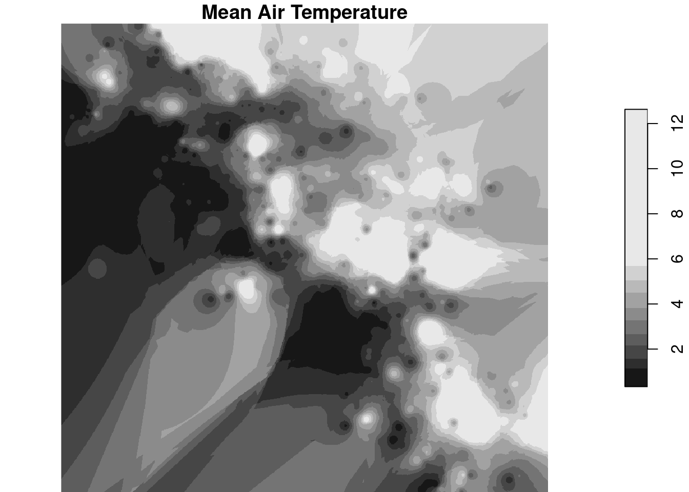
nmin (requirement to avoid contribution of fewer measurements)
nmax (local interpolation, reduce computation time)

Map_tmean <- idw( formula = Tmean~1,
                  locations = tmean_sf,
                  newdata = Campania_stars, 
                  nmin = 4,
                  nmax = 8
)
#> Warning in asMethod(object): complete map seems to be NA's
#> -- no selection was made
#> [inverse distance weighted interpolation]
#> Warning in asMethod(object): complete map seems to be NA's
#> -- no selection was made

Map_tmean
#> stars object with 2 dimensions and 2 attributes
#> attribute(s):
#>                 Min.  1st Qu.   Median     Mean  3rd Qu.
#> var1.pred  0.3353952 1.827006 3.283143 3.424935 4.790734
#> var1.var          NA       NA       NA      NaN       NA
#>                Max.   NA's
#> var1.pred  12.63161      0
#> var1.var         NA 685328
#> dimension(s):
#>   from  to  offset delta                refsys x/y
#> x    1 844  398275   200 WGS 84 / UTM zone 33N [x]
#> y    1 812 4592903  -200 WGS 84 / UTM zone 33N [y]

16.2.3.2 Plot IDW map

plot(Map_tmean["var1.pred"], main = "Mean Air Temperature")

16.2.3.3 IDW parameters

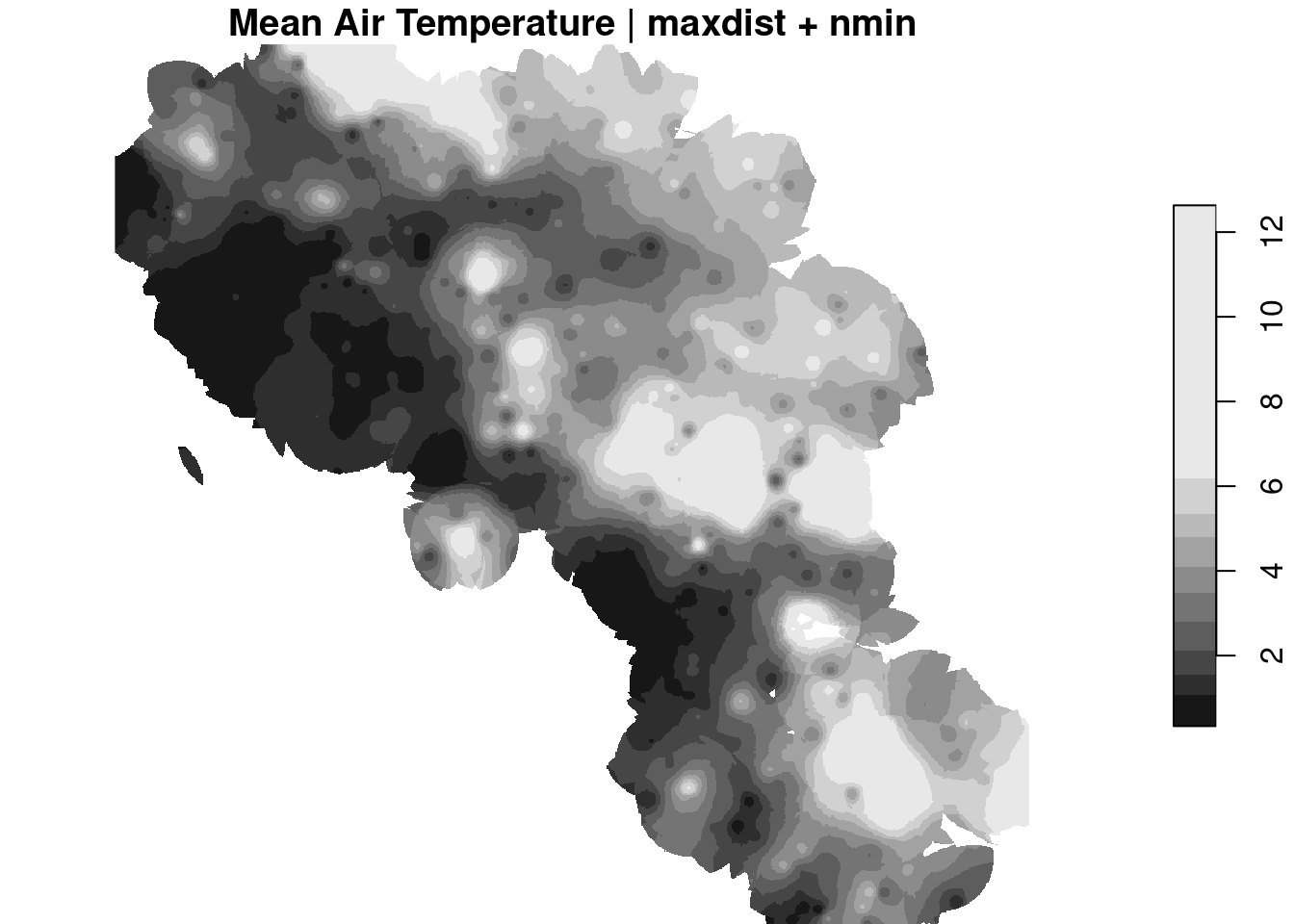
maxdist (radius of search for contributing measurements; nmin works only in combination of maxdist)

Map_tmean <- idw( formula = Tmean ~ 1,
                  locations = tmean_sf,
                  newdata = Campania_stars,
                  nmin = 4, 
                  nmax = 20,
                  maxdist = 10000)
#> Warning in asMethod(object): complete map seems to be NA's
#> -- no selection was made
#> [inverse distance weighted interpolation]
#> Warning in asMethod(object): complete map seems to be NA's
#> -- no selection was made

plot(Map_tmean, main = "Mean Air Temperature | maxdist + nmin")

15 Nearest Neighbours

17 Linear Regression