4 Vector Data Model

4.1 LINKS

sf package : Documentation of Package ‘sf’ [PDF]

4.2 Packages used

4.2.1 Install libraries

The following commands can be skipped in the RStudio instance provided by the teacher during the course.

install.packages("sf")
install.packages("raster")
install.packages("spData")
devtools::install_github("Nowosad/spDataLarge")
install.packages("osmdata")

Note: the installation of geojsonio can be sometimes tricky.

4.2.2 Load libraries

library(sf)          # classes and functions for vector data
library(raster)      # classes and functions for raster data
library(spData)      # load geographic data
library(spDataLarge) # load larger geographic data
library(osmdata)     # Open Street Map
library(kableExtra)  # see :: https://cran.r-project.org/web/packages/kableExtra/vignettes/awesome_table_in_html.html

4.3 An introduction to simple features

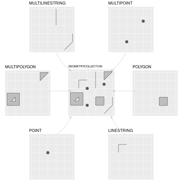
Figure 4.1: Simple Feature Geometries.

Simple features is an open standard developed and endorsed by the Open Geospatial Consortium (OGC), a not-for-profit organization (see Figure 4.1 for few examples).
Simple Features (SF) is a hierarchical data model that represents a wide range of geometry types.
Of 17 geometry types supported by the specification, only 7 are used in the vast majority of geographic research (see Figure below); these core geometry types are fully supported by the R package sf.

Geometries are the basic building blocks of simple features. Simple features in R can take on one of the 17 geometry types supported by the sf package. We will focus on the seven most commonly used types: POINT, LINESTRING, POLYGON, MULTIPOINT, MULTILINESTRING, MULTIPOLYGON, GEOMETRYCOLLECTION.

Find the whole list of possible feature types in the PostGIS manual.

The basis for each geometry type is the point.

A point is simply a coordinate in 2D, 3D or 4D space, from which the 7 geometry types can be derived:

POINT (5 2)
LINESTRING (1 5, 4 4, 4 1, 2 2, 3 2)
POLYGON ((1 5, 2 2, 4 1, 4 4, 1 5))
MULTIPOINT (5 2, 1 3, 3 4, 3 2)
MULTILINESTRING ((1 5, 4 4, 4 1, 2 2, 3 2), (1 2, 2 4))
MULTIPOLYGON (((1 5, 2 2, 4 1, 4 4, 1 5), (0 2, 1 2, 1 3, 0 3, 0 2)))
GEOMETRYCOLLECTION (MULTIPOINT (5 2, 1 3, 3 4, 3 2), LINESTRING (1 5, 4 4, 4 1, 2 2, 3 2))

4.3.1 Why simple features?

Because it is a widely supported data model that underlies data structures in many GIS applications including QGIS and PostGIS.
A major advantage of this is that using the data model ensures your work is cross-transferable to other set-ups, for example importing from and exporting to spatial databases.

vignette(package = "sf") # see which vignettes are available
vignette("sf1")          # an introduction to the package

4.4 Simple feature geometry (sfg)

Type	R sf function
A point:	st_point( )
A linestring:	st_linestring( )
A polygon:	st_polygon( )
A multipoint:	st_multipoint( )
A multilinestring:	st_multilinestring( )
A multipolygon:	st_multipolygon( )
A geometry collection:	st_geometrycollection( )

sfg objects can be created from three base R data types:

A numeric vector: a single point
A matrix: a set of points, where each row represents a point, a multipoint or linestring
A list: a collection of objects such as matrices, multilinestrings or geometry collections

(I have to make some examples about vector, matrix and list of points)

4.4.1 POINT

Create a POINT geometry and visualize it (Figure 4.2).

pt = st_point( c(5,2) )
class(pt)
#> [1] "XY"    "POINT" "sfg"
pt
#> POINT (5 2)

plot(pt,col="red",pch=16, cex=2)
axis(1,labels=T)
axis(2,labels=T)

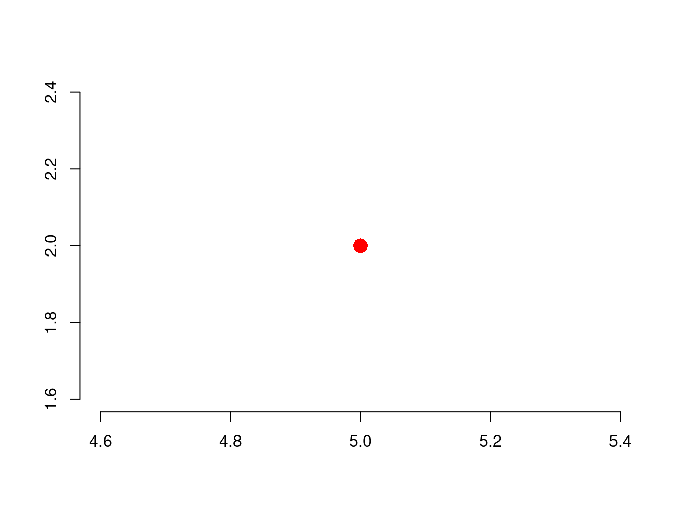
Figure 4.2: Example of POINT geometry.

4.4.2 LINESTRING

Create a matrix of 3 points connected by straight lines:

linestring_matrix = rbind( c(2,4), c(4,6), c(5,2) )
class( linestring_matrix )
#> [1] "matrix" "array"

Create a LINESTRING and visualize it (Figure 4.3).

ln = st_linestring( linestring_matrix )
class(ln)
#> [1] "XY"         "LINESTRING" "sfg"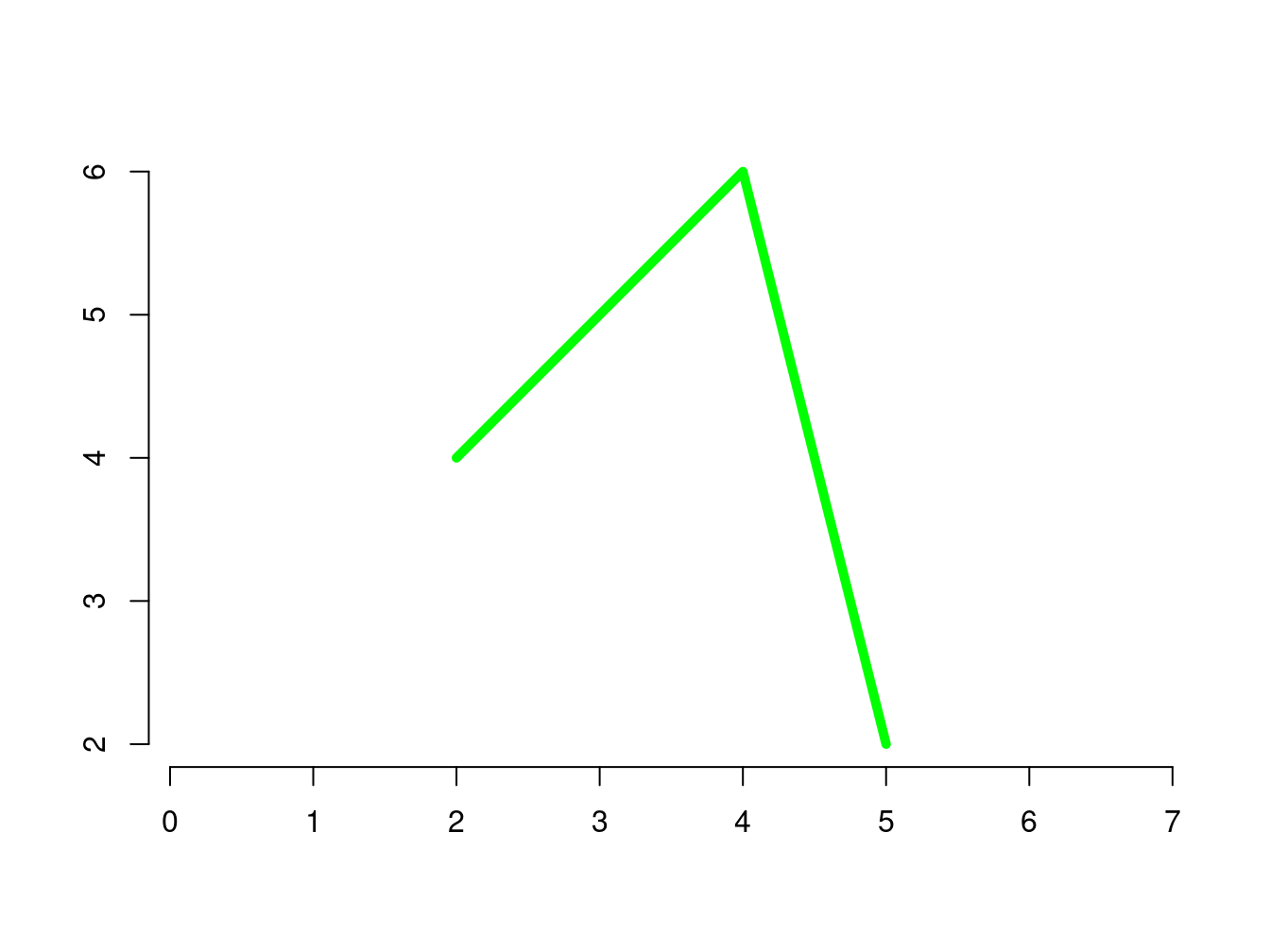

plot(ln,col="green", lwd=5)
axis(1,labels=T)
axis(2,labels=T)

Figure 4.3: Example of LINESTRING geometry.

4.4.3 POLYGON

Create a list of 4 points, in which the first and the last points are the same:

polygon_list = list(rbind( c(2,4), c(4,6), c(5,2) , c(2,4) ))
class( polygon_list )
#> [1] "list"

Create a POLYGON and visualize it (Figure 4.4).

pg = st_polygon( polygon_list )
class(pg)
#> [1] "XY"      "POLYGON" "sfg"

The polygon is made by same three points used in Figure 4.3, but 4 points are considered in the function above: why?
Because the first and the last points are identical.

plot(pg,col="yellow",lwd=5)
axis(1,labels=T)
axis(2,labels=T)

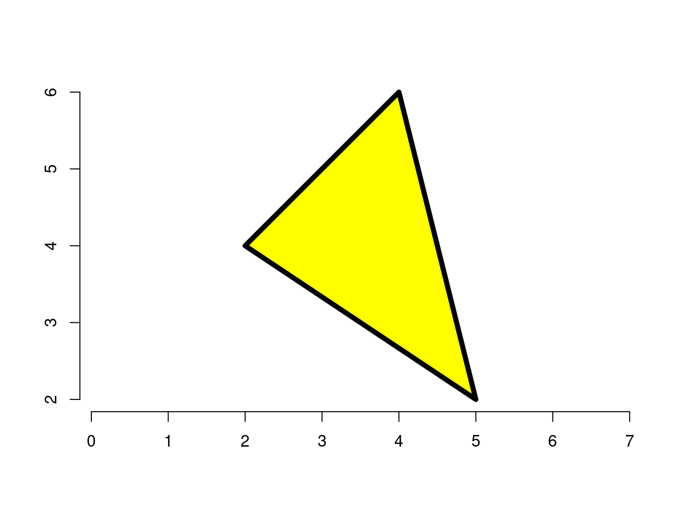
Figure 4.4: Example of POLYGON geometry.

4.4.4 MULTIPOINT

Create a matrix of 3 points:

multipoint_matrix = rbind( c(2,4) , c(4,6), c(5,2) )
class( multipoint_matrix )
#> [1] "matrix" "array"

Create a MULTIPOINT geometry and visualize it (Figure 4.5).

mp = st_multipoint( multipoint_matrix )
class(mp)
#> [1] "XY"         "MULTIPOINT" "sfg"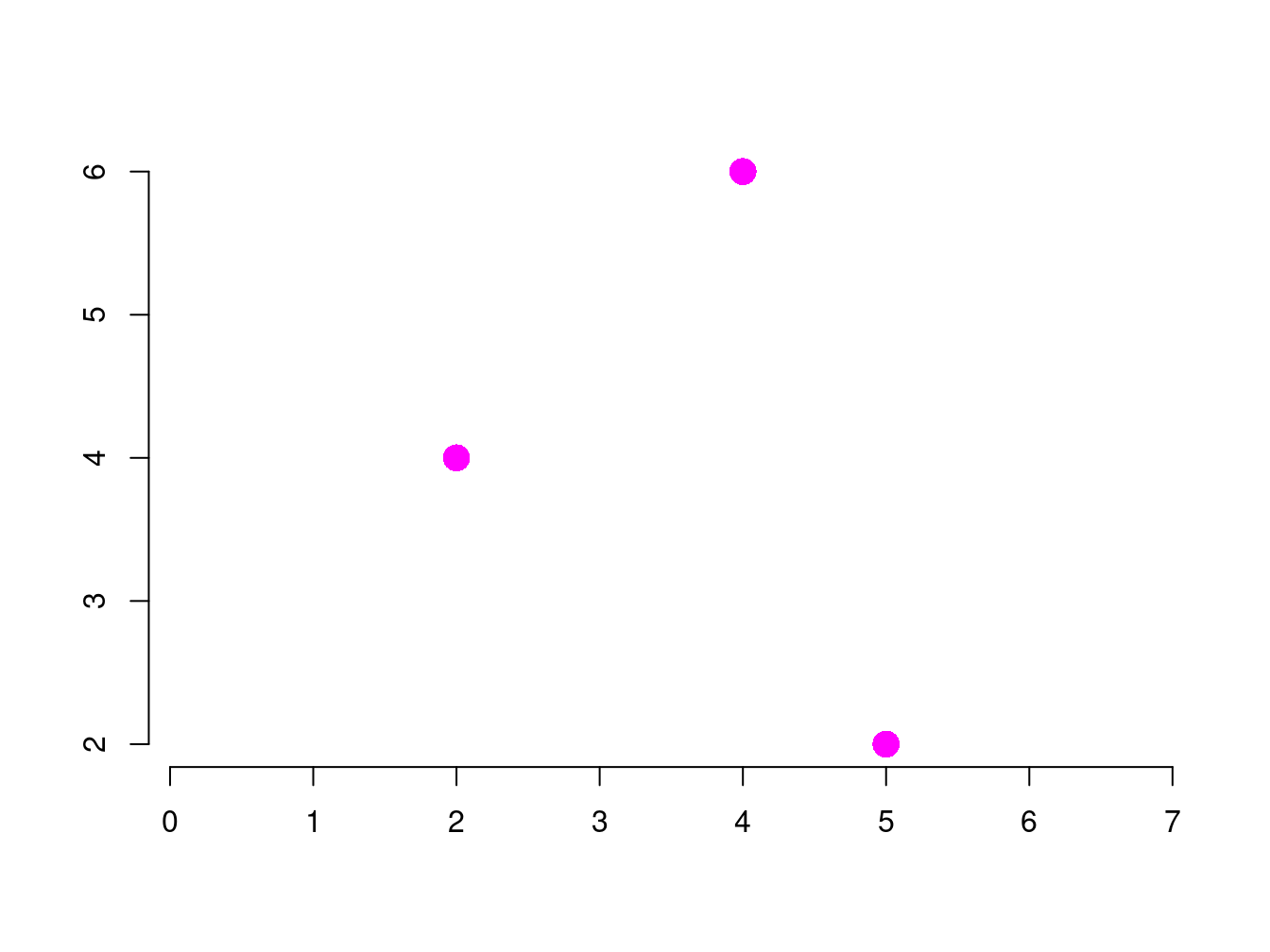

plot(mp,col="magenta", pch=16, cex=2)
axis(1,labels=T)
axis(2,labels=T)

Figure 4.5: Example of MULTIPOINT geometry.

The same set of points used for the LINESTRING (Figure 4.3) and POLYGON (Figure 4.4) is used.

4.4.5 MULTILINESTRING

Create a list of 10 points:

multilinestring_list = list( rbind( c(1, 5), c(2, 2), c(4, 1), c(4, 4) ) , 
                             rbind( c(0, 2), c(1, 2), c(1, 3), c(0, 3) ) 
                           )
class(multilinestring_list)
#> [1] "list"

Create a MULTILINESTRING geometry and visualize it (Figure 4.6).

mln = st_multilinestring( multilinestring_list )
class(mln)
#> [1] "XY"              "MULTILINESTRING" "sfg"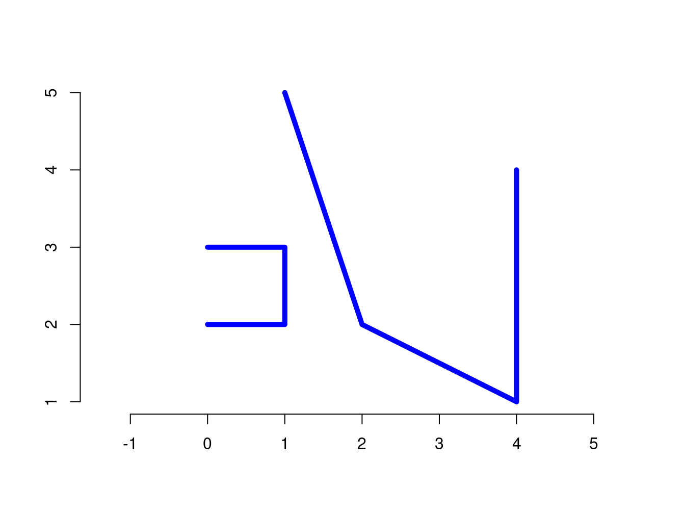

plot(mln,col="blue",lwd=5)
axis(1,labels=T)
axis(2,labels=T)

Figure 4.6: Example of MULTILINESTRING geometry.

4.4.6 MULTIPOLYGON

Create a nested list (i.e. list of list) of 10 points (the same points used in the MULTILINESTRING before, see Figure 4.6):

multipolygon_list = list(list( rbind(c(1, 5), c(2, 2), c(4, 1), c(4, 4), c(1, 5)) ),
                         list( rbind(c(0, 2), c(1, 2), c(1, 3), c(0, 3), c(0, 2)) )
                        )
class(multipolygon_list)
#> [1] "list"

Create a MULTIPOLYGON geometry and visualize it (Figure 4.7).

mpg = st_multipolygon( multipolygon_list )
class(mpg)
#> [1] "XY"           "MULTIPOLYGON" "sfg"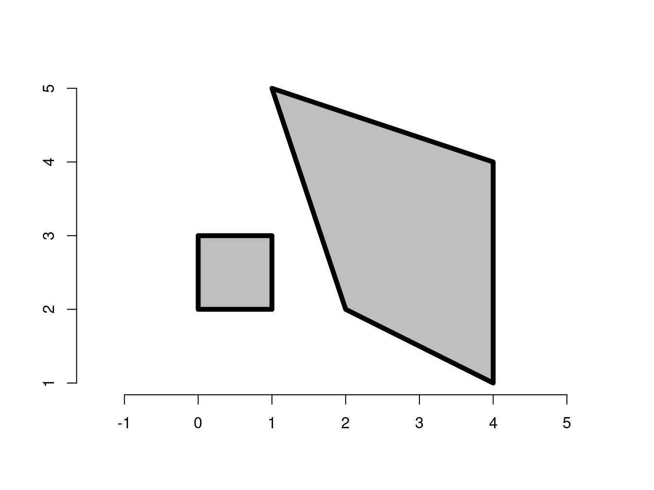

plot(mpg,col="gray",lwd=5)
axis(1,labels=T)
axis(2,labels=T)

Figure 4.7: Example of MULTIPOLYGON geometry.

4.4.7 GEOMETRYCOLLECTION

Create two matrices of 4 and 5 points:

multipoint_matrix = rbind(c(5, 2), c(1, 3), c(3, 4), c(3, 2))
linestring_matrix = rbind(c(1, 5), c(4, 4), c(4, 1), c(2, 2), c(3, 3))
class(multipoint_matrix)
#> [1] "matrix" "array"
class(linestring_matrix)
#> [1] "matrix" "array"

Create a GEOMETRYCOLLECTION geometry fusing a MULTIPOINT and a LINESTRING together:

geometrycollection_list = list(st_multipoint(multipoint_matrix),
                              st_linestring(linestring_matrix))
gcoll = st_geometrycollection(geometrycollection_list)
class(gcoll)
#> [1] "XY"                 "GEOMETRYCOLLECTION"
#> [3] "sfg"

Visualze it:

plot(gcoll,col="violet",pch=16,cex=2,lwd=5)
axis(1,labels=T)
axis(2,labels=T)

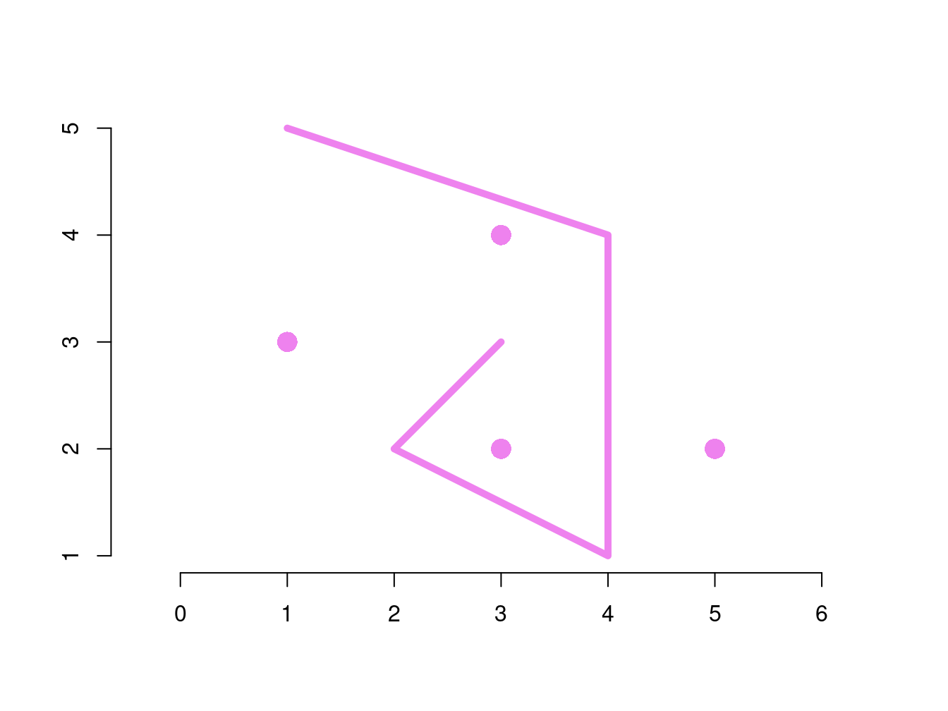
Figure 4.8: Example of GEOMETRYCOLLECTION geometry.

What is the geometry type?

st_geometry_type(gcoll)
#> [1] GEOMETRYCOLLECTION
#> 18 Levels: GEOMETRY POINT LINESTRING POLYGON ... TRIANGLE

4.5 Simple features column (sfc)

Think about the requirement of a soil survey in which we need to observe two soil profiles in the field. We have to collect soil samples from the topsoil and then carry out laboratory analysis to retrieve physical and chemical soil properties. The first step is to select the localization of the two points, which means that we can attach to each geospatial point two coordinates given by our GPS device. For instance, using simple coordinates for the sake of clarity:

Soil Profile ID	Geospatial Coordinates (x,y)
\(P_1\)	(5,2)
\(P_2\)	(1,3)

We can create two POINT geometries as follows:

P1 = st_point(c(5, 2))
P2 = st_point(c(1, 3))

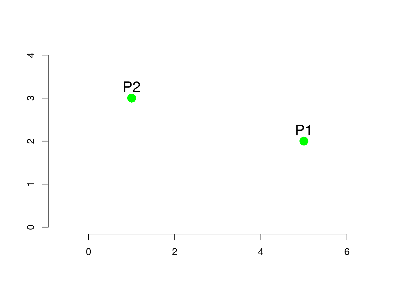
How can we create an object in which collecting the geospatial location of the soil profiles?

4.5.1 From pure geometry of distinct POINTs to a set of organized records (SFG)

One sfg object contains only a single simple feature geometry.

A simple feature geometry column (sfc) can collect more sfg objects:

points_sfc = st_sfc(P1, P2)
class(points_sfc)
#> [1] "sfc_POINT" "sfc"

Print in R console the metadata associated to the SFC object:

print(points_sfc)
#> Geometry set for 2 features 
#> Geometry type: POINT
#> Dimension:     XY
#> Bounding box:  xmin: 1 ymin: 2 xmax: 5 ymax: 3
#> CRS:           NA
#> POINT (5 2)
#> POINT (1 3)

In addition, as you can see in the print above, the sfc can manage also the information about the Coordinate Reference System (CRS) in use. In the command above st_sfc(P1, P1) we didn’t set the CRS and the st_sfc() function has a dedicated argument to do this, e.g. st_sfc(..., crs=4326).

A Simple Feature Column (SFC) can be built for any collection of geometry types.

In the following example, two records representing two forest patches are listed together to get a SFG:

# Forest Patch #1, e.g. Pinus
polygon_list1 = list(rbind(c(1, 5), c(2, 2), c(4, 1), c(4, 4), c(1, 5)))
polygon1 = st_polygon(polygon_list1)
# Forest Patch #2, e.g. Quercus
polygon_list2 = list(rbind(c(0, 2), c(1, 2), c(1, 3), c(0, 3), c(0, 2)))
polygon2 = st_polygon(polygon_list2)
# SFG
polygon_sfc = st_sfc(polygon1, polygon2)
print(polygon_sfc)
#> Geometry set for 2 features 
#> Geometry type: POLYGON
#> Dimension:     XY
#> Bounding box:  xmin: 0 ymin: 1 xmax: 4 ymax: 5
#> CRS:           NA
#> POLYGON ((1 5, 2 2, 4 1, 4 4, 1 5))
#> POLYGON ((0 2, 1 2, 1 3, 0 3, 0 2))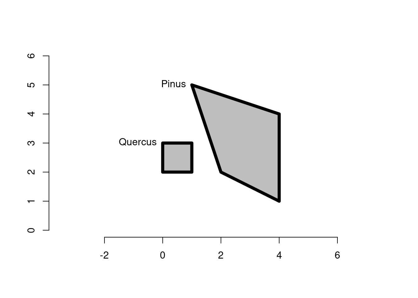

plot(polygon_sfc, col="gray", lwd=5, xlim=c(-1,5), ylim=c(0,6))

Figure 4.9: Two forest patches managed using a SFC.

It is also possible to create a SFC object from a set of SFG having different geometry types:

# combining objects created above:
mixed_sfc = st_sfc(P1, mln, polygon1)
# plot:
plot(mixed_sfc, pch=16, cex=2, lwd=5)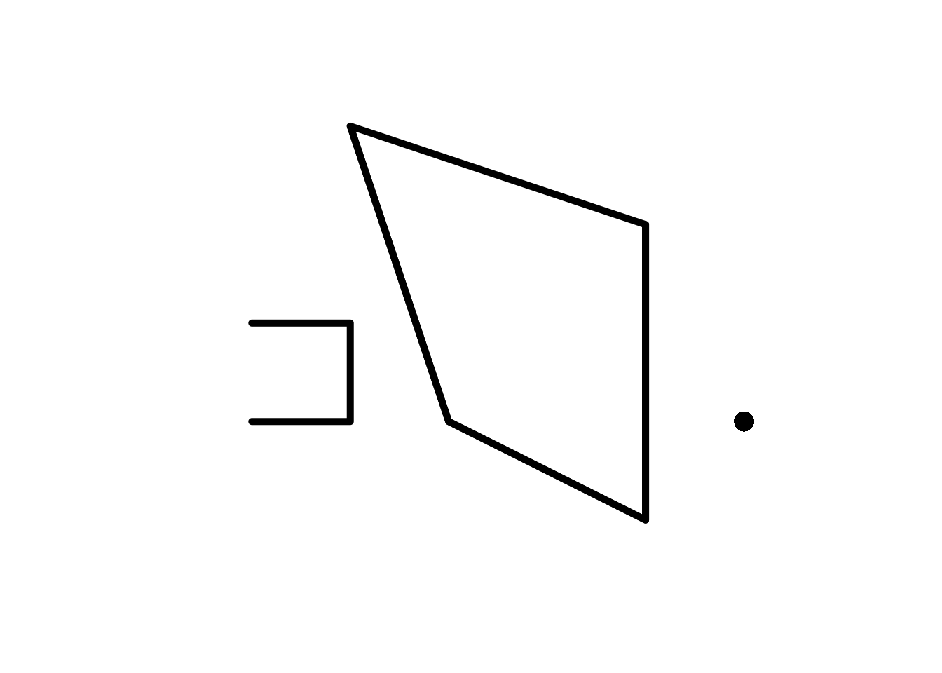

4.5.2 CRS (Coordinate Reference System)

SFC objects can additionally store information on the coordinate reference systems (CRS).
To specify a certain CRS, we can use the EPSG (SRID) or proj4string attributes of an sfc object.

print(points_sfc)
#> Geometry set for 2 features 
#> Geometry type: POINT
#> Dimension:     XY
#> Bounding box:  xmin: 1 ymin: 2 xmax: 5 ymax: 3
#> CRS:           NA
#> POINT (5 2)
#> POINT (1 3)

The default value of EPSG (SRID) and proj4string is NA (Not Available), as can be verified with the function st_crs( ):

st_crs(points_sfc)
#> Coordinate Reference System: NA

The argument crs is used to set the Reference System in use by the coordinates. In our simple example, we assume GCS (Geodetic Coordinate reference System) in which the points \(P_1\) and \(P_2\) have geographical coordinates Longitude and Latitude (WGS84 datum):

# EPSG definition
points_sfc_wgs = st_sfc(P1, P2, crs = 4326)
print(points_sfc_wgs)
#> Geometry set for 2 features 
#> Geometry type: POINT
#> Dimension:     XY
#> Bounding box:  xmin: 1 ymin: 2 xmax: 5 ymax: 3
#> Geodetic CRS:  WGS 84
#> POINT (5 2)
#> POINT (1 3)

A detailed reading of the CRS is made:

st_crs(points_sfc_wgs)
#> Coordinate Reference System:
#>   User input: EPSG:4326 
#>   wkt:
#> GEOGCRS["WGS 84",
#>     ENSEMBLE["World Geodetic System 1984 ensemble",
#>         MEMBER["World Geodetic System 1984 (Transit)"],
#>         MEMBER["World Geodetic System 1984 (G730)"],
#>         MEMBER["World Geodetic System 1984 (G873)"],
#>         MEMBER["World Geodetic System 1984 (G1150)"],
#>         MEMBER["World Geodetic System 1984 (G1674)"],
#>         MEMBER["World Geodetic System 1984 (G1762)"],
#>         MEMBER["World Geodetic System 1984 (G2139)"],
#>         ELLIPSOID["WGS 84",6378137,298.257223563,
#>             LENGTHUNIT["metre",1]],
#>         ENSEMBLEACCURACY[2.0]],
#>     PRIMEM["Greenwich",0,
#>         ANGLEUNIT["degree",0.0174532925199433]],
#>     CS[ellipsoidal,2],
#>         AXIS["geodetic latitude (Lat)",north,
#>             ORDER[1],
#>             ANGLEUNIT["degree",0.0174532925199433]],
#>         AXIS["geodetic longitude (Lon)",east,
#>             ORDER[2],
#>             ANGLEUNIT["degree",0.0174532925199433]],
#>     USAGE[
#>         SCOPE["Horizontal component of 3D system."],
#>         AREA["World."],
#>         BBOX[-90,-180,90,180]],
#>     ID["EPSG",4326]]

4.6 The SF class

A ‘SF Geometry’ object is purely geometric and a ‘SF Column’ object is a geographic building block.
In order to create a SF we need to fulfil the following steps:

Create two SFG, e.g. POINT geometry (\(P_1\) and \(P_2\)) (add a link here to the section).
Create a SFC, e.g. collect together \(P_1\) and \(P_2\) and define a CRS (add a link here to the section).
Create a table of attributes (or variables) by means of which real-world entities can be described and create a Simple Feature (SF) st_sf( ).

4.6.1 Creation of a Simple Feature

A simple feature can be created:

from scratch
- using synthetic data
- using real-world data
from a vector data model stored in a
- local file
- remote file

4.6.1.1 From scratch | synthetic data

Let’s build an example from scratch.

Step 01: create purely geometric objects.

P1_sfg = st_point(c(5, 2))
P2_sfg = st_point(c(1, 3))
print(P1_sfg)
#> POINT (5 2)

Step 02: create a geospatial object

P_sfc <- st_sfc(P1_sfg, P2_sfg, crs=4326)
print(P_sfc)
#> Geometry set for 2 features 
#> Geometry type: POINT
#> Dimension:     XY
#> Bounding box:  xmin: 1 ymin: 2 xmax: 5 ymax: 3
#> Geodetic CRS:  WGS 84
#> POINT (5 2)
#> POINT (1 3)

Step 03: add attributes Real-world entities, such as soils, have measurable characteristics that can be stored in attributes or variables.
The third and final building block to get a SF is the creation of these non-geographic attributes.

attrib <- data.frame( clay = c(25,47), sand = c(30,23), silt = c(45,30) )
P_sf <- st_sf(attrib,P_sfc)
print(P_sf)
#> Simple feature collection with 2 features and 3 fields
#> Geometry type: POINT
#> Dimension:     XY
#> Bounding box:  xmin: 1 ymin: 2 xmax: 5 ymax: 3
#> Geodetic CRS:  WGS 84
#>   clay sand silt       P_sfc
#> 1   25   30   45 POINT (5 2)
#> 2   47   23   30 POINT (1 3)

In the above R object we have all the information, both data and metadata, required to fully describe a Simple Feature as defined by the OGC Standard.

The vector data model created for the simple example above can be managed in R but also exported to be managed in whatever software capable of GIS funcionalities.

(NOTE: create a new example -> forest or livestock)

4.6.1.2 From scratch | real-world data

In this example we read data from files which are not designed to implement any vector data model.
The temperature and precipitation measurements carried out by standard agrometeorological ground stations are extracted from Excel files (Excel format is not the best interoperable practice):

Both the measurements and the geolocalization tables are used in the reading / import below:

require(readxl)
#> Loading required package: readxl
Tmax   <- read_excel("Tmax.xlsx", sheet = "measurements", na = "NA")
Rain   <- read_excel("Rainfall.xlsx", sheet = "measurements", na = "NA")
lonlat <- read_excel("Tmax.xlsx", sheet = "geolocalization", na = "NA")

Table 4.1: Here is a preview of the daily maximum Air Temperatura measurements.
DATE	MODENAURB	SAGATABOAGRO	ZOLAPREDOSAAGRO	RAVARINO	CORREGGIOAGRO
2007-01-01	6.5	7.0	8.4	NA	6.6
2007-01-02	10.9	10.0	10.5	NA	12.5
2007-01-03	13.3	12.9	13.5	NA	13.4
2007-01-04	9.5	7.0	7.6	NA	7.0
2007-01-05	10.5	11.9	10.5	NA	10.3

Table 4.2: Here is a preview of the daily cumulative Rainfall measurements.
DATE	MODENAURB	SAGATABOAGRO	CORREGGIOAGRO	ZOLAPREDOSAAGRO
2007-01-01	0.0	0.0	0.0	0.0
2007-01-02	0.4	0.4	0.0	1.6
2007-01-03	0.0	0.0	0.2	0.0
2007-01-04	0.0	0.0	0.0	0.0
2007-01-05	0.0	0.0	0.0	0.0

Table 4.3: The coordinates in the geodetic reference system WGS84 (EPSG:4326).
Station	Longitude	Latitude
MODENAURB	10.91571	44.65191
SAGATABOAGRO	11.13887	44.68841
ZOLAPREDOSAAGRO	11.19870	44.48924
RAVARINO	11.10133	44.71573
CORREGGIOAGRO	10.76922	44.73740

Extract coordinates, temperature and rainfall measurements for MODENAURB station on 2007-01-01:

name <- lonlat$Station[1]
t1   <- Tmax$MODENAURB[1]
r1   <- Rain$MODENAURB[1]
d1   <- Tmax$DATE[1]
lon  <- lonlat$Longitude[1]
lat  <- lonlat$Latitude[1]
print( c(name, lon,lat,t1,r1) )
#> [1] "MODENAURB" "10.91571"  "44.65191"  "6.5"      
#> [5] "0"

Create a Simple Feature using the values extracted above:

point   = st_point(c(lon, lat))        # 1. sfg object
class(point)                           #    see that the class is a sfg
#> [1] "XY"    "POINT" "sfg"
geom    = st_sfc(point, crs = 4326)    # 2. sfc object
class(geom)                            #    see that the class is a sfc
#> [1] "sfc_POINT" "sfc"
attrib  = data.frame(                  # 3. attributes
   name = name,                        #    Station name, "MODENAURB"
   date = as.Date(d1),                 #    Convert the date-time in date, on '2007-01-01'
   temperature = t1,                   #    Air Temperature for "MODENAURB" on '2007-01-01'
   rainfall = r1                       #    Rainfall for "MODENAURB" on '2007-01-01'
)
# Simple Feature (Collection):
SF = st_sf(attrib, geometry = geom)    # 3. sf object
class(SF)                              #    see that the class is a sf
#> [1] "sf"         "data.frame"
print(SF)                              #    see both metadata and data in the simple feature
#> Simple feature collection with 1 feature and 4 fields
#> Geometry type: POINT
#> Dimension:     XY
#> Bounding box:  xmin: 10.91571 ymin: 44.65191 xmax: 10.91571 ymax: 44.65191
#> Geodetic CRS:  WGS 84
#>        name       date temperature rainfall
#> 1 MODENAURB 2007-01-01         6.5        0
#>                    geometry
#> 1 POINT (10.91571 44.65191)

In the example provided above, only one record was created but it is possible to add more records (or features) belonging to both other stations and other dates.

The list of variable / attributes / fields (in this handbook the term variable is prefered):

names(SF)
#> [1] "name"        "date"        "temperature" "rainfall"   
#> [5] "geometry"

Print the geometry only:

print(SF$geometry)
#> Geometry set for 1 feature 
#> Geometry type: POINT
#> Dimension:     XY
#> Bounding box:  xmin: 10.91571 ymin: 44.65191 xmax: 10.91571 ymax: 44.65191
#> Geodetic CRS:  WGS 84
#> POINT (10.91571 44.65191)

4.6.1.3 Interchange format | local file

Load the air temperature measurements carried out by the standard agrometeorological ground stations (IoT context):

t_day <- read.csv("AirTemperature_day.csv")

Table 4.4: A preview of the Air Temperature data frame
Name	lon	lat	elev	mean	min	max	N
Acerra 26	14.42840	40.96617	26	12.482518	9.6	13.7	143
Airola 154	14.59057	41.07170	154	10.090909	7.7	11.3	77
Alife	14.33372	41.33922	117	12.315972	9.1	14.1	144
Alife 152	14.28492	41.34177	152	12.113986	9.4	13.9	143
Altavilla Irpina	14.78386	41.00628	352	8.765972	5.0	11.1	144
Alvignano	14.39467	41.21825	235	10.397917	7.2	12.2	144
Apice 597	14.97204	41.12760	597	6.366197	3.1	9.9	142
Ariano Irpino	15.08542	41.14853	678	5.808333	3.1	8.0	144
Auletta	15.42831	40.55181	194	9.980556	3.7	13.6	144
Avellino Genio Civile	14.78358	40.91197	360	9.108333	6.3	10.9	144

class(t_day)
#> [1] "data.frame"

Convert a data frame into a simple feature (see the new field geometry created by the function st_as_sf()):

t_day_sf <- st_as_sf(t_day,coords = c("lon","lat"), crs=4326)

Table 4.5: A preview of the Air Temperature simple feature
Name	elev	mean	min	max	N	geometry
Acerra 26	26	12.482518	9.6	13.7	143	POINT (14.4284 40.96617)
Airola 154	154	10.090909	7.7	11.3	77	POINT (14.59057 41.0717)
Alife	117	12.315972	9.1	14.1	144	POINT (14.33372 41.33922)
Alife 152	152	12.113986	9.4	13.9	143	POINT (14.28492 41.34177)
Altavilla Irpina	352	8.765972	5.0	11.1	144	POINT (14.78386 41.00628)
Alvignano	235	10.397917	7.2	12.2	144	POINT (14.39467 41.21825)
Apice 597	597	6.366197	3.1	9.9	142	POINT (14.97204 41.1276)
Ariano Irpino	678	5.808333	3.1	8.0	144	POINT (15.08542 41.14853)
Auletta	194	9.980556	3.7	13.6	144	POINT (15.42831 40.55181)
Avellino Genio Civile	360	9.108333	6.3	10.9	144	POINT (14.78358 40.91197)

4.6.1.4 Existing Vector Data Model | local file

Import in R the Improsta Farm Digital Soil Map. The st_read() function reads a vector data model written in Shapefile format:

require(sf)
imp_dsm <- st_read("DigitalSoilMap_Improsta.shp")
#> Reading layer `DigitalSoilMap_Improsta' from data source 
#>   `/home/giuliano/datasets/vector/DigitalSoilMap_Improsta.shp' 
#>   using driver `ESRI Shapefile'
#> Simple feature collection with 20 features and 8 fields
#> Geometry type: POLYGON
#> Dimension:     XY
#> Bounding box:  xmin: 496825.7 ymin: 4488864 xmax: 498998.6 ymax: 4489958
#> Projected CRS: WGS 84 / UTM zone 33N

Table 4.6: A preview of the Improsta farm digital soil map
N_UC	SIGLA_UC	SIGLA_DEL	COD_AM	Area	Area_ha	Irriga_ca1	geometry
9	RIS0	RIS0.1	NA	31725.85	3	3, bassa	POLYGON ((497213.9 4489528,…
3	PIN0	PIN0.1	NA	36894.60	4	2, media	POLYGON ((497875.7 4489750,…
4	CAM0	CAM0.1	NA	27920.44	3	2, media	POLYGON ((497796.7 4489646,…
5	ERB0	ERB0.1	NA	77809.70	8	3, bassa	POLYGON ((497867.8 4489410,…
6	ERB1	ERB1.1	NA	13630.73	1	3, bassa	POLYGON ((497117.8 4489411,…

plot(imp_dsm["SIGLA_UC"], axes=TRUE, border="grey")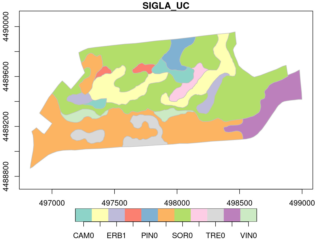

Figure 4.10: Digital Soil Map of Telese Valley.

4.6.1.5 Existing Vector Data Model | remote data source

The getbb() function can search in OpenStreetMap using a toponym (e.g. Emilia Romagna) and can return a simple feature as output (format_out=sf_polygon):

require(osmdata)
ER  = osmdata::getbb("Emilia Romagna",format_out="sf_polygon")
names(ER)
#> [1] "polygon"      "multipolygon"
ER <- ER$multipolygon

In section creating data from scratch we created the SF simple feature from scratch:

SF # or print(SF)
#> Simple feature collection with 1 feature and 4 fields
#> Geometry type: POINT
#> Dimension:     XY
#> Bounding box:  xmin: 10.91571 ymin: 44.65191 xmax: 10.91571 ymax: 44.65191
#> Geodetic CRS:  WGS 84
#>        name       date temperature rainfall
#> 1 MODENAURB 2007-01-01         6.5        0
#>                    geometry
#> 1 POINT (10.91571 44.65191)

plot(ER$geometry,reset=F)
plot(SF$geometry,add=T,pch=16,col="red")
axis(1, labels=TRUE)
axis(2, labels=TRUE)
text( st_coordinates(SF), 'MODENAURB', pos=2 )
title( xlab="Longitude [degree]", ylab="Latitude [degree]" )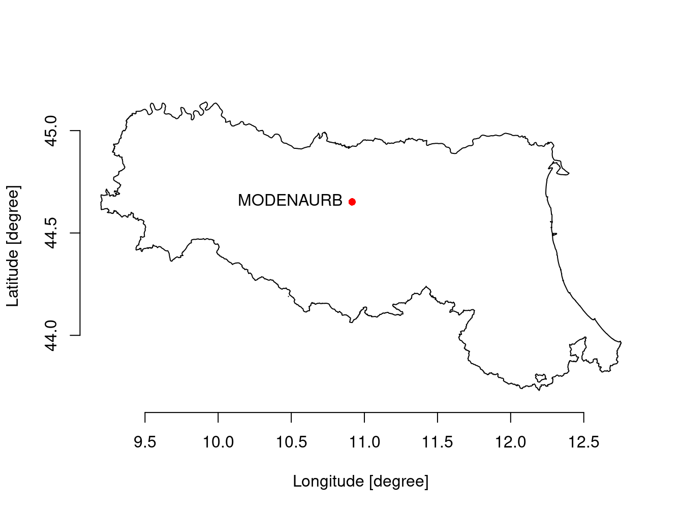

Figure 4.11: Emilia Romagna Region with MODENAURB station.

4.6.2 Export a Simple Feature

In section creating data from scratch we created the SF simple feature from scratch.

SF # or print(SF)
#> Simple feature collection with 1 feature and 4 fields
#> Geometry type: POINT
#> Dimension:     XY
#> Bounding box:  xmin: 10.91571 ymin: 44.65191 xmax: 10.91571 ymax: 44.65191
#> Geodetic CRS:  WGS 84
#>        name       date temperature rainfall
#> 1 MODENAURB 2007-01-01         6.5        0
#>                    geometry
#> 1 POINT (10.91571 44.65191)

Let’s export / save / write it to a file using a standard vector data model/driver (e.g. geojson format):

st_write(SF,"my_first_simple_feature.geojson")

Note that the driver used to write data on HDD depends on the file extension provided: in the example above, it was used .geojson but any other extension can be used.

4.6.3 Vector drivers / formats

Here follows the list of drivers that are available in the current GDAL installation:

name	long_name	write	copy	is_raster	is_vector	vsi
ESRIC	Esri Compact Cache	FALSE	FALSE	TRUE	TRUE	TRUE
FITS	Flexible Image Transport System	TRUE	FALSE	TRUE	TRUE	FALSE
PCIDSK	PCIDSK Database File	TRUE	FALSE	TRUE	TRUE	TRUE
netCDF	Network Common Data Format	TRUE	TRUE	TRUE	TRUE	TRUE
PDS4	NASA Planetary Data System 4	TRUE	TRUE	TRUE	TRUE	TRUE
VICAR	MIPL VICAR file	TRUE	TRUE	TRUE	TRUE	TRUE
JP2OpenJPEG	JPEG-2000 driver based on OpenJPEG library	FALSE	TRUE	TRUE	TRUE	TRUE
PDF	Geospatial PDF	TRUE	TRUE	TRUE	TRUE	TRUE
MBTiles	MBTiles	TRUE	TRUE	TRUE	TRUE	TRUE
BAG	Bathymetry Attributed Grid	TRUE	TRUE	TRUE	TRUE	TRUE
EEDA	Earth Engine Data API	FALSE	FALSE	FALSE	TRUE	FALSE
OGCAPI	OGCAPI	FALSE	FALSE	TRUE	TRUE	TRUE
ESRI Shapefile	ESRI Shapefile	TRUE	FALSE	FALSE	TRUE	TRUE
MapInfo File	MapInfo File	TRUE	FALSE	FALSE	TRUE	TRUE
UK .NTF	UK .NTF	FALSE	FALSE	FALSE	TRUE	TRUE
LVBAG	Kadaster LV BAG Extract 2.0	FALSE	FALSE	FALSE	TRUE	TRUE
OGR_SDTS	SDTS	FALSE	FALSE	FALSE	TRUE	TRUE
S57	IHO S-57 (ENC)	TRUE	FALSE	FALSE	TRUE	TRUE
DGN	Microstation DGN	TRUE	FALSE	FALSE	TRUE	TRUE
OGR_VRT	VRT - Virtual Datasource	FALSE	FALSE	FALSE	TRUE	TRUE
REC	EPIInfo .REC	FALSE	FALSE	FALSE	TRUE	FALSE
Memory	Memory	TRUE	FALSE	FALSE	TRUE	FALSE
CSV	Comma Separated Value (.csv)	TRUE	FALSE	FALSE	TRUE	TRUE
NAS	NAS - ALKIS	FALSE	FALSE	FALSE	TRUE	TRUE
GML	Geography Markup Language (GML)	TRUE	FALSE	FALSE	TRUE	TRUE
GPX	GPX	TRUE	FALSE	FALSE	TRUE	TRUE
LIBKML	Keyhole Markup Language (LIBKML)	TRUE	FALSE	FALSE	TRUE	TRUE
KML	Keyhole Markup Language (KML)	TRUE	FALSE	FALSE	TRUE	TRUE
GeoJSON	GeoJSON	TRUE	FALSE	FALSE	TRUE	TRUE
GeoJSONSeq	GeoJSON Sequence	TRUE	FALSE	FALSE	TRUE	TRUE
ESRIJSON	ESRIJSON	FALSE	FALSE	FALSE	TRUE	TRUE
TopoJSON	TopoJSON	FALSE	FALSE	FALSE	TRUE	TRUE
Interlis 1	Interlis 1	TRUE	FALSE	FALSE	TRUE	TRUE
Interlis 2	Interlis 2	TRUE	FALSE	FALSE	TRUE	TRUE
OGR_GMT	GMT ASCII Vectors (.gmt)	TRUE	FALSE	FALSE	TRUE	TRUE
GPKG	GeoPackage	TRUE	TRUE	TRUE	TRUE	TRUE
SQLite	SQLite / Spatialite	TRUE	FALSE	FALSE	TRUE	TRUE
ODBC		FALSE	FALSE	FALSE	TRUE	FALSE
WAsP	WAsP .map format	TRUE	FALSE	FALSE	TRUE	TRUE
PGeo	ESRI Personal GeoDatabase	FALSE	FALSE	FALSE	TRUE	FALSE
MSSQLSpatial	Microsoft SQL Server Spatial Database	TRUE	FALSE	FALSE	TRUE	FALSE
OGR_OGDI	OGDI Vectors (VPF, VMAP, DCW)	FALSE	FALSE	FALSE	TRUE	FALSE
PostgreSQL	PostgreSQL/PostGIS	TRUE	FALSE	FALSE	TRUE	FALSE
MySQL	MySQL	TRUE	FALSE	FALSE	TRUE	FALSE
OpenFileGDB	ESRI FileGDB	FALSE	FALSE	FALSE	TRUE	TRUE
DXF	AutoCAD DXF	TRUE	FALSE	FALSE	TRUE	TRUE
CAD	AutoCAD Driver	FALSE	FALSE	TRUE	TRUE	TRUE
FlatGeobuf	FlatGeobuf	TRUE	FALSE	FALSE	TRUE	TRUE
Geoconcept	Geoconcept	TRUE	FALSE	FALSE	TRUE	TRUE
GeoRSS	GeoRSS	TRUE	FALSE	FALSE	TRUE	TRUE
GPSTrackMaker	GPSTrackMaker	TRUE	FALSE	FALSE	TRUE	TRUE
VFK	Czech Cadastral Exchange Data Format	FALSE	FALSE	FALSE	TRUE	FALSE
PGDUMP	PostgreSQL SQL dump	TRUE	FALSE	FALSE	TRUE	TRUE
OSM	OpenStreetMap XML and PBF	FALSE	FALSE	FALSE	TRUE	TRUE
GPSBabel	GPSBabel	TRUE	FALSE	FALSE	TRUE	FALSE
OGR_PDS	Planetary Data Systems TABLE	FALSE	FALSE	FALSE	TRUE	TRUE
WFS	OGC WFS (Web Feature Service)	FALSE	FALSE	FALSE	TRUE	TRUE
OAPIF	OGC API - Features	FALSE	FALSE	FALSE	TRUE	FALSE
SOSI	Norwegian SOSI Standard	FALSE	FALSE	FALSE	TRUE	FALSE
Geomedia	Geomedia .mdb	FALSE	FALSE	FALSE	TRUE	FALSE
EDIGEO	French EDIGEO exchange format	FALSE	FALSE	FALSE	TRUE	TRUE
SVG	Scalable Vector Graphics	FALSE	FALSE	FALSE	TRUE	TRUE
CouchDB	CouchDB / GeoCouch	TRUE	FALSE	FALSE	TRUE	FALSE
Cloudant	Cloudant / CouchDB	TRUE	FALSE	FALSE	TRUE	FALSE
Idrisi	Idrisi Vector (.vct)	FALSE	FALSE	FALSE	TRUE	TRUE
ARCGEN	Arc/Info Generate	FALSE	FALSE	FALSE	TRUE	TRUE
XLS	MS Excel format	FALSE	FALSE	FALSE	TRUE	FALSE
ODS	Open Document/ LibreOffice / OpenOffice Spreadsheet	TRUE	FALSE	FALSE	TRUE	TRUE
XLSX	MS Office Open XML spreadsheet	TRUE	FALSE	FALSE	TRUE	TRUE
Elasticsearch	Elastic Search	TRUE	FALSE	FALSE	TRUE	FALSE
Walk		FALSE	FALSE	FALSE	TRUE	FALSE
Carto	Carto	TRUE	FALSE	FALSE	TRUE	FALSE
AmigoCloud	AmigoCloud	TRUE	FALSE	FALSE	TRUE	FALSE
SXF	Storage and eXchange Format	FALSE	FALSE	FALSE	TRUE	TRUE
Selafin	Selafin	TRUE	FALSE	FALSE	TRUE	TRUE
JML	OpenJUMP JML	TRUE	FALSE	FALSE	TRUE	TRUE
PLSCENES	Planet Labs Scenes API	FALSE	FALSE	TRUE	TRUE	FALSE
CSW	OGC CSW (Catalog Service for the Web)	FALSE	FALSE	FALSE	TRUE	FALSE
VDV	VDV-451/VDV-452/INTREST Data Format	TRUE	FALSE	FALSE	TRUE	TRUE
GMLAS	Geography Markup Language (GML) driven by application schemas	FALSE	TRUE	FALSE	TRUE	TRUE
MVT	Mapbox Vector Tiles	TRUE	FALSE	FALSE	TRUE	TRUE
NGW	NextGIS Web	TRUE	TRUE	TRUE	TRUE	FALSE
MapML	MapML	TRUE	FALSE	FALSE	TRUE	TRUE
TIGER	U.S. Census TIGER/Line	TRUE	FALSE	FALSE	TRUE	TRUE
AVCBin	Arc/Info Binary Coverage	FALSE	FALSE	FALSE	TRUE	TRUE
AVCE00	Arc/Info E00 (ASCII) Coverage	FALSE	FALSE	FALSE	TRUE	TRUE
HTTP	HTTP Fetching Wrapper	FALSE	FALSE	TRUE	TRUE	FALSE

4.6.3.1 Exercise

Annotate the drivers from the list that you already know.

3 Geospatial Data

5 Raster Data Model