17 Linear Regression
17.1 Notes
See also the example in the Interoperability & FAIR chapter in which a WCPS query to rasdaman endpoint is shown.
17.3 Application: Air temperature vs Elevation
An example using the D.E.M. (Digital Elevation Model) raster follows.
See Wikipedia article on
Atmospheric Temperature for more details.
17.3.1 Problem definition
We can expect the air temperature to decrease by 6.5 degrees Celsius for every 1000 meters you gain in elevation.
It means that for every meter we move up in elevation, the temperature decreases by 6.5/1000 °C:
6.5/1000
#> [1] 0.0065
The slope (\(\beta\)) of the relationship between temperature and elevation is 0.0065 Celsius degrees per each meter:
\(\beta = -0.0065 \frac{[°C]}{[m]}\)
17.3.2 Make a prediction
If we assume a temperature of 0 °C at elevation 0 meters…
elev <- 0  # a.s.l. above see level
t0 <- 0  # *C
beta <- -0.0065
…what is the predicted temperature at elevation given in the raster dem at index position (1,1)?
First, import the raster DEM in R:
dem <- rast("../datasets/raster/dem5m_vt.tif")…and then extract / read the value from the pixel requested above:
dem[1, 1]
#>   dem5m_vt
#> 1    217.7
Now, predict the temperature value for this pixel:
t <- 0 + 217.7 * -0.0065
print(t)
#> [1] -1.41505
The R command above can be also written as:
t <- t0 + dem[1, 1] * beta
print(t)
#>   dem5m_vt
#> 1 -1.4150517.3.4 Expand our model
Objective: make predictions of temperature using the information about elevation.
We assume a linear regression model of the form:
\(y = \alpha + \beta x\)
Now, assume a temperature of 12.5 °C at elevation 0 meters (the \(\alpha\) parameter of the model) for today:
\(\alpha = 12.5 \;°C\)
Calculate / Predict the value of temperature at positions in the DEM where matrix indices are:
- (1,1)
dem[1, 1]
#>   dem5m_vt
#> 1    217.7
12.5 - 0.0065 * dem[1, 1]
#>   dem5m_vt
#> 1 11.08495- (200,700)
dem[200, 700]
#>   dem5m_vt
#> 1    784.2
12.5 - 0.0065 * dem[200, 700]
#>   dem5m_vt
#> 1 7.4027- (3200,2200)
dem[3200, 2200]
#>   dem5m_vt
#> 1   1182.4
12.5 - 0.0065 * dem[3200, 2200]
#>   dem5m_vt
#> 1   4.8144
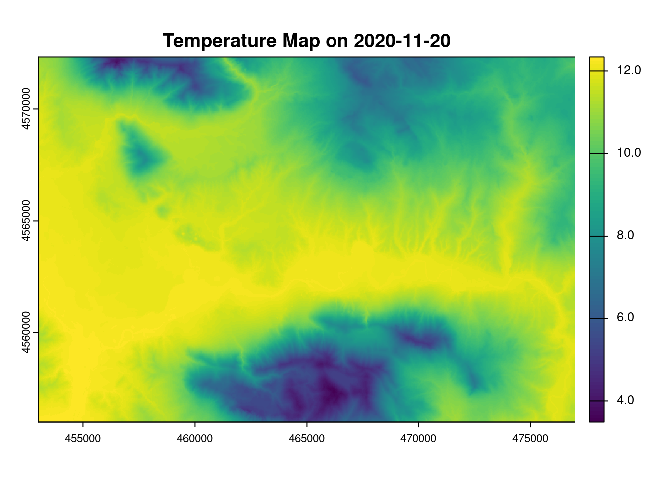
17.3.4.1 Estimate the temperature on the whole raster
How can we extend the calculation made on one pixel to every pixels in the raster?
a <- 12.5           # alpha
b <- -0.0065        # beta
T <- a + b * dem    # temperature
Print the content:
T
#> class       : SpatRaster
#> size        : 3264, 4800, 1  (nrow, ncol, nlyr)
#> resolution  : 5, 5  (x, y)
#> extent      : 453000, 477000, 4556000, 4572320  (xmin, xmax, ymin, ymax)
#> coord. ref. : WGS 84 / UTM zone 33N (EPSG:32633)
#> source(s)   : memory
#> varname     : dem5m_vt
#> name        : dem5m_vt
#> min value   :  3.48580
#> max value : 12.3966517.3.6 Save raster | temperature map
writeRaster( x = T,
             filename = "Tair_VT_20201120.tif",
             overwrite = TRUE
           )
See which GDAL raster drivers are available in GDAL and which one are installed within your R environment using the command given in section Raster drivers / formats.
