11 Spatial Variability
11.1 Foundations of geostatistical modelling: reality, uncertainty, and observations
11.1.1 Reality
Reality is deterministic.
The real spatial field exists and is defined for every location
\[
z(s), \quad s \in A
\]
The real field is determined by physical processes.
Typical examples are clay content, rainfall, soil organic matter.
However, \[ Z(s) \neq z(s) \]
In geostatistics we do not work directly with reality, but with a statistical model of reality, denoted by \(Z(s)\).
The stochastic process does not describe reality itself, but our uncertainty about the world.
11.1.2 From reality to observations
In practice, we never observe the real field
\[
z(s), \quad s \in A
\]
What we actually have are measurements, taken at a finite number of locations.
Measurements are affected by error, due to instruments, sampling procedures, and small-scale variability that we do not resolve.
Therefore, at each sampled location \(s\), we observe
\[ Y(s) = z(s) + e(s) \]
where:
- \(Y(s)\) is the observed value,
- \(z(s)\) is the true (but unknown) value of the real field,
- \(e(s)\) is the measurement error.
The error term \(e(s)\) is typically assumed to have zero mean and finite variance.
This does not mean that the world is random, but that our access to it is imperfect.
11.1.3 The stochastic process \(Z(s)\): introducing the random variable concept
Since \(z(s)\) is unknown everywhere except at the sampled points (and even there only imperfectly), we need a way to represent our uncertainty about its value.
This is done by introducing a random variable \(Z(s)\).
At each location \(s \in A\), \(Z(s)\) represents the possible values that the real field \(z(s)\) could take, given what we know.
For simplicity, and motivated by the Central Limit Theorem, we often assume that
\[ Z(s) \sim \mathcal{N}(\mu, \sigma^2) \]
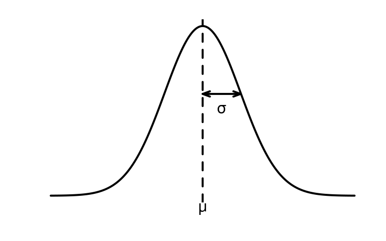
That is:
- the distribution of \(Z(s)\) is normal,
- with mean \(\mu\),
- and variance \(\sigma^2\).
Importantly:
- \(Z(s)\) is not the reality,
- it is a probabilistic description of our uncertainty about reality at location \(s\).
At this stage, uncertainty is described at a single location only.
To proceed toward geostatistics, we must still describe how \(Z(s)\) and \(Z(s')\) are related in space.
11.2 Understanding Spatial Variability
In a completely random world, we could imagine every point on a map — say, temperature readings at different places — having its own dice. You roll the dice at each location independently. So, even if two points are just a few meters apart, their values might be completely unrelated. This is what we call white noise — randomness with no memory of space.
But nature doesn’t behave like that.
In the real world, things that are close in space tend to be similar. If it’s warm here, it’s probably warm just next to it. If the soil is wet at one point, it will likely be moist a meter away too. This spatial smoothness is a key idea.
So, instead of imagining a bunch of dice being rolled independently at each point, imagine something like a stretchy surface, like a soft blanket. When you push down on it in one place (a low value), the area around it dips too — not as much, but a little. Likewise, a bump in one place raises the surrounding area a bit.
This blanket is our random field:
- It still contains randomness — every place has uncertainty.
- But this randomness is structured in space — nearby points are related.
From here, we start building assumptions:
- How strongly do values at different points relate?
- How far does that influence go?
- How quickly does similarity fade with distance?
These assumptions define the model of spatial dependence, which forms the foundation for how we simulate, interpolate, or predict values in space.
In nature, things aren’t completely random — they vary in a structured way across space. That brings us to the idea of a random field:
at each location \(\mathbf{s}_i\), there is a random variable.
But these variables are not completely independent — they’re linked by space.
11.2.1 Properties of a Random Function \(Z(\mathbf{s})\)
We can now ask: what properties should this random function have?
11.2.1.1 1. Defined everywhere in space
We want to be able to say, “What’s the value of the variable at this location?” — for any point on the map.
Meaning:
The random function \(Z(\mathbf{s})\) assigns a random variable to every location \(\mathbf{s}\) in a region \(D \subset \mathbb{R}^2\).
11.2.1.2 2. Each point has uncertainty
Even if we don’t know the exact value at a point, we assume it follows a distribution — typically Gaussian.
Meaning:
At each location \(\mathbf{s}_i\), we have a random variable \(Z(\mathbf{s}_i)\) with a mean and a variance — representing the expected value and its possible deviation.
11.2.1.3 3. Nearby points are more similar
If two points are close, they tend to have similar values; if they’re far apart, they may differ substantially.
Meaning:
This is the principle of spatial autocorrelation — the core of spatial modeling.
We typically express it using a function that describes how similarity decays with distance.
11.2.1.4 4. Same behavior everywhere (optional)
Sometimes we assume that the field behaves the same way in every direction and at every place — an assumption that simplifies modeling.
Meaning:
This leads to two common properties:
-
Stationarity — the rules don’t change depending on where you are.
- Isotropy — the rules don’t change depending on which direction you look.
These are simplifying assumptions, but very common starting points for spatial models.
11.2.2 The Covariance Function (or Structure Function)
Now that we have assumed:
-
Stationarity — the statistical behavior is the same everywhere;
- Isotropy — the statistical behavior is the same in every direction;
we can describe the field’s spatial dependence entirely through how similar values are at different distances apart.
11.2.2.1 Definition
The covariance function captures this dependence:
Let:
-
\(Z(\mathbf{s})\): the value at location \(\mathbf{s}\)
- \(\text{Cov}(h) = \text{Cov}(Z(\mathbf{s}), Z(\mathbf{s+h}))\)
If the field is stationary and isotropic, then:
\[ \text{Cov}(Z(\mathbf{s}), Z(\mathbf{s+h})) = C(h) \]
This means that the covariance depends only on the distance \(h = \|\mathbf{h}\|\), not on position or direction.
11.2.2.2 Common Forms of \(C(h)\)
| Model | Formula | Interpretation |
|---|---|---|
| Exponential | \(C(h) = \sigma^2 \exp(-h/a)\) | Rapid decay, short-range correlation |
| Gaussian | \(C(h) = \sigma^2 \exp(-(h/a)^2)\) | Very smooth field |
| Spherical | Piecewise-defined up to a cutoff | Finite correlation distance |
Parameters:
-
\(\sigma^2\): sill — total variance
- \(a\): range — distance at which correlation becomes negligible
11.2.3 Why This Matters
- Enables the generation of random fields (e.g., via Cholesky decomposition)
- Allows prediction of missing values (kriging)
- Provides a framework to fit models to spatial data
11.2.4 Stationarity and Isotropy
When we say that a random field is stationary, we mean that the statistical properties of the field don’t change with location.
In other words, no matter where you are, the distribution of values behaves in the same way.
More precisely, under second-order stationarity:
- The mean is constant: \[ \mathbb{E}[Z(\mathbf{s})] = \mu, \quad \forall \mathbf{s} \]
- The variance is constant: \[ \text{Var}[Z(\mathbf{s})] = \sigma^2, \quad \forall \mathbf{s} \]
- The covariance depends only on the separation vector \(\mathbf{h}\): \[ \text{Cov}(Z(\mathbf{s}), Z(\mathbf{s+h})) = C(\mathbf{h}) \]
When we say that a random field is isotropic, we mean that the spatial dependence is identical in every direction.
Thus, the covariance depends only on distance: \[ C(\mathbf{h}) = C(h), \quad \text{with } h = \|\mathbf{h}\| \]
That is, two points 5 m apart have the same correlation whether they are east–west, north–south, or diagonal — same distance ⇒ same dependence.
11.2.5 In Summary
-
Stationarity → Local statistics (mean, variance, covariance) are the same everywhere.
- Isotropy → Spatial relationships are the same in every direction.
These assumptions greatly simplify both modeling and estimation, and they are often a reasonable first approximation of real spatial data.
11.3 Understanding Random Fields and Their Statistical Distribution
A random field is a function that assigns a random variable to every location in space. In the spatial context, we can think of a random field as a map of values, each of which is the outcome of a random process occurring at a specific location.
Formally, a random field \(Z(\mathbf{s})\) is defined over a domain \(\mathbf{s} \in D \subset \mathbb{R}^2\), where each location \(\mathbf{s} = (x, y)\) has a corresponding random variable.

Figure 11.1: A random field \(Z(\mathbf{s})\) defined over a spatial domain \(D \subset \mathbb{R}^2\). Each black point represents a spatial location \(\mathbf{s}_i\), to which a random variable \(Z(\mathbf{s}_i)\) is associated. Selected locations display their probability distribution, illustrating that the field is composed of spatially indexed random variables.
Didactic notes on the figure:
- The use of a regular grid with black dots effectively represents a discrete spatial domain over which a spatial process is defined.
- The vertically emerging bell-shaped curves emphasize that each location \(\mathbf{s}_i\) is associated with a random variable \(Z(\mathbf{s}_i)\), governed by a probability distribution.
- The notation \(Z(\mathbf{s})\) refers to the random field as a whole — a spatial function mapping each location to a random variable — while \(Z(\mathbf{s}_i)\) denotes the random variable at a specific point.
- Only a subset of these random variables is explicitly visualized, reinforcing that the field is defined over the entire domain, not just the displayed points.
- The coordinate notation is \(\mathbf{s}_1 = (x_1, y_1)\), which clarifies that each location belongs to the spatial domain \(D \subset \mathbb{R}^2\).
- At location \(\mathbf{s}_1\), the figure highlights the probabilistic selection of a specific value from the bell-shaped curve (gaussian distribution) using a dashed line. This single outcome, \(z(\mathbf{s}_1)\), is called a regionalized value — the observed value of the random variable \(Z(\mathbf{s}_1)\) at that location.
- Extending this idea to all locations in the spatial domain, the set of regionalized values \(\{z(\mathbf{s}_i)\}\) forms a regionalized variable \(z(\mathbf{s})\). It represents a spatially continuous (or discrete) field of observed values (observed field) that stems from a single realization of the underlying random field \(Z(\mathbf{s})\).
- Each bell-shaped curve represents the full probability distribution of the random variable \(Z(\mathbf{s}_i)\), not just a single value. While we observe only one outcome (the regionalized value), conceptually, many realizations are possible — and their average would converge to the mean of the distribution.
We typically assume that the field is second-order stationary, meaning that:
The mean is constant across space: \[ \mathbb{E}[Z(\mathbf{s})] = \mu, \quad \forall\; \mathbf{s} \]
The variance is constant: \[ \text{Var}(Z(\mathbf{s})) = \sigma^2, \ \forall\; \mathbf{s} \]
The covariance between any two locations depends only on the separation vector \(h = \|\mathbf{s}_1 - \mathbf{s}_2\|\) (and not on the absolute position): \[ \text{Cov}(Z(\mathbf{s}_1), Z(\mathbf{s}_2)) = C(\mathbf{h}), \ \text{where} \ \mathbf{h} = \mathbf{s}_1 - \mathbf{s}_2 \]
And if you further assume isotropy, then: \[ C(\mathbf{h}) = C(\|\mathbf{h}\|) \] i.e. the covariance depends only on the distance, not the direction.
When modeling such fields, we often assume that the random variables follow a Gaussian distribution. This implies that the entire field \(Z\) is a realization of a multivariate normal distribution:
\[ Z \sim \mathcal{N}(\boldsymbol{\mu}, \mathbf{C}) \]
where:
- \(\boldsymbol{\mu}\) is the mean vector (often constant),
- \(\mathbf{C}\) is the covariance matrix derived from the spatial covariance function (e.g., exponential, spherical).
A particularly important case is the white noise field, where the random variables are independent and identically distributed (i.i.d.):
\[ Z(\mathbf{s}) \overset{\text{i.i.d.}}{\sim} \mathcal{N}(0, \sigma^2) \]
In this case, the covariance matrix \(\mathbf{C}\) reduces to a diagonal matrix — and no spatial structure is present.
Later, we will introduce spatially correlated random fields, where nearby values are similar due to a structured covariance. These spatial dependencies give rise to rich patterns that we can simulate and analyze.
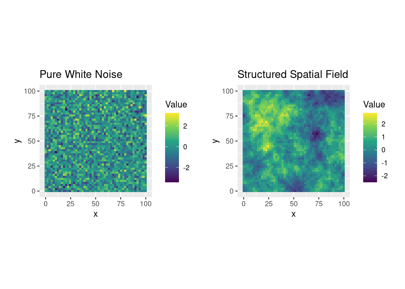
Figure 11.2: Two random fields: one with no spatial structure (left) and one with evident spatial correlation (right).
11.4 Introducing Spatial Correlation
In a purely random field, the value at each location is independent of its neighbors. However, many natural processes — including soil properties, elevation, or temperature — tend to vary gradually in space, meaning that nearby values are more similar than distant ones (Tobler’s Law). This phenomenon is called spatial autocorrelation.
11.4.1 Spatial Covariance Matrix
To represent spatial correlation mathematically, we use a covariance matrix \(\mathbf{C}\), where each element \(C_{ij}\) describes how strongly the value at location \(\mathbf{s}_i\) is correlated with the value at location \(\mathbf{s}_j\).
For a stationary and isotropic process, the covariance depends only on the distance \(h = \|\mathbf{s}_i - \mathbf{s}_j\|\), not on the absolute position or direction. That is:
\[ C_{ij} = C(h) = \text{Cov}(Z(\mathbf{s}_i), Z(\mathbf{s}_j)) = \sigma^2 \cdot \rho(h) \]
where:
- \(\sigma^2\) is the variance of the process (also called the sill),
- \(\rho(h)\) is the correlation function (e.g., exponential, spherical), which decays with distance.
Note:
Given two observed values of a variable at spatial locations \(\mathbf{s}_1\) and \(\mathbf{s}_2\),
say \(Z(\mathbf{s}_1) = 0.12\) and \(Z(\mathbf{s}_2) = 0.10\), and the mean \(\bar{Z} = 0.11\),
the sample covariance is:
\[ \text{Cov}(Z(\mathbf{s}_1), Z(\mathbf{s}_2)) = (0.12 - 0.11)(0.10 - 0.11) = -0.001 \]
A common choice is the exponential model:
\[ \rho(h) = \exp\left(-\frac{h}{r}\right) \]
Here, \(r\) is the range parameter, which determines how quickly correlation drops with distance. For instance, if \(h = r\), then the correlation between two points is \(\approx 0.37\).
11.4.2 Simulating Spatial Fields from a Covariance Matrix
To simulate a spatial field with this correlation structure, we follow these steps:
- Build the covariance matrix \(\mathbf{C}\) using the chosen correlation function
- Decompose the matrix using Cholesky decomposition: \[ \mathbf{C} = \mathbf{L} \mathbf{L}^\top \]
- Generate a vector of independent Gaussian noise: \[ \mathbf{G} \sim \mathcal{N}(\mathbf{0}, \mathbf{I}) \]
- Multiply to create a spatially correlated field: \[ \mathbf{Z} = \mathbf{L} \cdot \mathbf{G} \]
The result is a realization of a Gaussian random field with spatial correlation. Visually, the field appears smooth, with values transitioning gradually over space.
11.4.3 Comparison
| Property | Pure Random Field | Spatially Correlated Field |
|---|---|---|
| Covariance Matrix | Diagonal (no correlation) | Full matrix (distance-dependent) |
| Visual Appearance | Grainy, noisy | Smooth, continuous patterns |
| Mathematical Structure | \(\mathbf{Z} \sim \mathcal{N}(\mathbf{0}, \sigma^2 \mathbf{I})\) | \(\mathbf{Z} \sim \mathcal{N}(\mathbf{0}, \mathbf{C})\) |
11.5 Simulating Spatial Fields: From Theory to Practice
- Briefly recap the idea that we can now generate fields with and without structure.
- Introduce the simulation approach using covariance functions and Cholesky decomposition.
- Include the actual simulation plots (as you already created).
- Highlight how changing the range or sill alters the visual structure.
To better understand how spatial correlation shapes the structure of a random field, we can simulate artificial spatial data with and without correlation. This hands-on approach helps reveal how theory translates into visible spatial patterns.
We use a Gaussian random field model, where the spatial dependence is encoded through a covariance matrix \(\mathbf{C}\). By applying the Cholesky decomposition, we can generate realizations that follow this prescribed structure.
11.5.1 Step-by-Step Procedure
- Define a grid of spatial locations \(\mathbf{s}_1, \mathbf{s}_2, \ldots, \mathbf{s}_n\).
# Grid definition
n <- 50
grid <- expand.grid(x = seq(0, 100, length.out = n),
y = seq(0, 100, length.out = n))- Compute all pairwise distances to form a distance matrix.
-
Build the covariance matrix \(\mathbf{C}\) using a chosen correlation model, such as the exponential:
\[
C(h) = \sigma^2 \cdot \exp\left( -\frac{h}{r} \right)
\]
where:
- \(\sigma^2\) is the variance (sill),
- \(r\) is the range,
- \(h\) is the distance between two locations.
# Covariance function
cov_function <- function(sill, range, h) {
  sill * exp(-h / range)
}- Apply the Cholesky decomposition: \[ \mathbf{C} = \mathbf{L} \mathbf{L}^\top \] where \(\mathbf{L}\) is a lower triangular matrix.
# Structured field: covariance matrix and Cholesky
sill <- 1
range <- 20
C <- cov_function(sill, range, h = dist_matrix)
L <- chol(C)- Generate independent standard normal values: \[ \mathbf{G} \sim \mathcal{N}(\mathbf{0}, \mathbf{I}) \]
- Construct the correlated field: \[ \mathbf{Z} = \mathbf{L} \cdot \mathbf{G} \]
z_structured <- crossprod(L, G)-
Generate the uncorrelated field with matching variance:
This field is composed of independent values drawn from a normal distribution with the same variance as the correlated field (i.e., the sill), allowing for a fair comparison. \[ \mathbf{Z}_\text{random} \sim \mathcal{N}(0, \sigma^2), \quad \text{with } \sigma^2 = \text{sill} \]
# Random field: pure nugget with same variance as structured field
set.seed(678)
z_random <- rnorm(nrow(grid), 0, sqrt(sill))
This vector \(\mathbf{Z}\) represents a realization of a spatially correlated process. We can compare it to a white noise field (no spatial correlation), where each location receives a value drawn independently from the same normal distribution.
11.5.2 Visual Example
Below are two simulated spatial fields over the same grid:
- Left: a pure white noise field (no spatial correlation)
- Right: a structured field with exponential spatial correlation
library(ggplot2)
library(patchwork)
library(viridis)
library(gridExtra)

# Prepare data for plotting
df <- grid
df$structured <- as.numeric(z_structured)
df$random <- z_random

# Plot
p1 <- ggplot(df, aes(x, y, fill = random)) +
  geom_raster() +
  coord_equal() +
  scale_fill_viridis_c() +
  labs(title = "Pure White Noise", fill = "Value")

p2 <- ggplot(df, aes(x, y, fill = structured)) +
  geom_raster() +
  coord_equal() +
  scale_fill_viridis_c() +
  labs(title = "Spatially Correlated Field", fill = "Value")

grid.arrange(p1, p2, ncol = 2)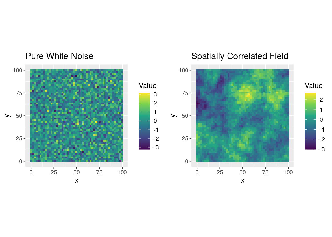
Figure 11.3: Comparison between white noise and a spatially structured random field
As we can see, the spatially structured field exhibits continuity, with values changing gradually over space, unlike the grainy appearance of white noise.
This experiment shows how a well-defined covariance model creates smoothness, and how the range parameter controls the scale of spatial dependence.
11.6 Decomposing a Spatial Field into Components
Introduce the conceptual idea of trend + structure + noise
Define:
\(\mu(\mathbf{s})\): deterministic trend
\(S(\mathbf{s})\): spatially correlated residual
\(\varepsilon(\mathbf{s})\): nugget or white noisez
Relate this to physical/geographical phenomena (e.g., SOC increases with altitude but with local variability).
In many real-world applications, a spatial variable is not entirely random. Its spatial variability can often be explained as the sum of three conceptually distinct components:
\[Z(\mathbf{s}) = \mu(\mathbf{s}) + S(\mathbf{s}) + \varepsilon(\mathbf{s})\] where:
- \(\mu(\mathbf{s})\) is the trend component, often driven by known environmental covariates (e.g., coordinates, elevation);
- \(S(\mathbf{s})\) is the structured residual, accounting for spatial autocorrelation not explained by the trend;
- \(\varepsilon(\mathbf{s})\) is a spatial white noise term, including the nugget effect, i.e., micro-scale variation and measurement noise.
This decomposition is central in geostatistics and spatial modeling because each component has a different origin and must be handled accordingly.
Before delving into the mathematical details of each component of a spatial random field, an illustrative example is here provided. The figure below shows the simulated decomposition of a spatial field into:
- a deterministic trend depending on spatial coordinates and elevation,
- a short-range spatial structure capturing local continuity,
- a long-range spatial structure capturing broad-scale variation,
- a spatial white noise component is often introduced in simulations to represent local variability that is uncorrelated in space. While part of this unstructured variation may correspond to the nugget effect — such as measurement error or unresolved micro-scale variation — it can also include other forms of high-frequency noise that are not captured by the structured spatial model.
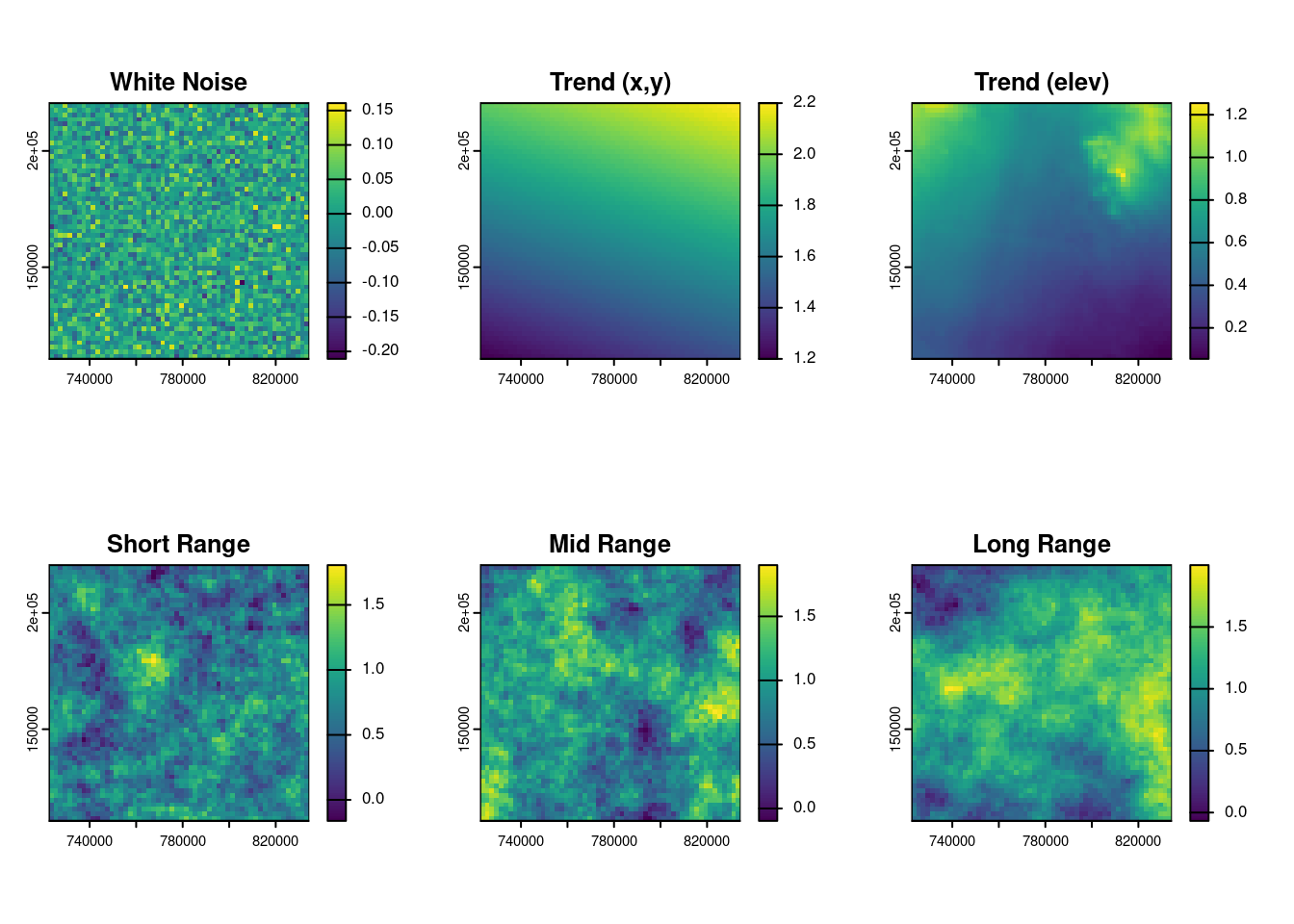
Figure 11.4: Compponents of the spatial field.
The final simulated field is obtained as the sum of these components. This visual decomposition helps build intuition on how spatial variability arises from both structured and unstructured sources.
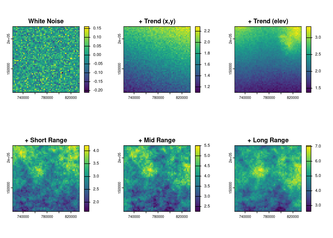
Figure 11.5: From noise to structure: the relative contribution of spatial components.
11.6.1 Trend Component: Large-Scale Variation
The trend represents the deterministic part of the spatial field. It captures gradual, systematic changes over space and may depend on covariates such as elevation or location:
\[ \mu(\mathbf{s}) = \beta_0 + \beta_1 x + \beta_2 y + \beta_3 z \] This component explains long-range variation — for instance, an increasing soil property with altitude or a west-to-east gradient.
11.6.2 Structured Residual: Spatial Dependence
The residual component \(S(\mathbf{s})\) represents the spatially correlated part of the variation that is not explained by the trend. It captures medium- to short-range dependence, such as clusters of similar values.
This component is modeled via a covariance function and often simulated using Cholesky decomposition, as shown earlier.
11.6.3 Nugget Effect: Random Noise
The nugget \(\varepsilon(\mathbf{s})\) models purely uncorrelated random noise. It may reflect measurement error or spatial variability occurring at scales finer than our sampling resolution.
Visually, this component introduces local “graininess” into the spatial field.
11.6.4 Summary Table
| Component | Description | Spatial Scale | Statistical Nature |
|---|---|---|---|
| \(\mu(\mathbf{s})\) | Deterministic trend (e.g. slope, elevation) | Long-range | Known function |
| \(S(\mathbf{s})\) | Structured residual | Medium/short-range | Random, correlated |
| \(\varepsilon(\mathbf{s})\) | Micro-scale variability or error | Very short-range | Random, uncorrelated |
This decomposition enables a structured approach to modeling spatial variability, where each component is estimated, modeled, or simulated according to its nature.